DiscoveringStatsUsingR
本书章节对应年级(英制)
| Chapter | 1st year undergraduate | 2nd year undergraduate | Post-graduates | |
|---|---|---|---|---|
| 1 | ✓ | |||
| 2 | ✓ | |||
| 3 | ✓ | |||
| 4 | ✓ | |||
| 5 | ✓ | ✓ | ||
| 6 | ✓ | |||
| 7 | ✓ | |||
| 8 | ✓ | |||
| 9 | ✓ | |||
| 10 | ✓ | |||
| 11 | ✓ | |||
| 12 | ✓ | |||
| 13 | ✓ | |||
| 14 | ✓ | |||
| 15 | ✓ | |||
| 16 | ✓ | |||
| 17 | ✓ | |||
| 18 | ✓ | |||
| 19 | ✓ | |||
| Levels | ① | ② ③ | ③ ④ |
BODMAS 运算顺序
- B: ()
- O: order, 阶数,序;如平方 42
- D:
- M:
- A: +
- S: -
C1. Why to learn statistics?
从提出研究问题到分析数据
graph TD

A[Research questions]--> B1[data]
A[Research questions]--> B2[提出theory]

B2 -->|需要quantify| C[提出hypothesis]
C -->|需要确定测量的变量vars| C1[收数据、检验theory]
C --> C2[identify vars]
	C1 --> D[分析数据]
	C1 --> E[measure vars]
	C2 --> C3(自变量,因变量)
D --> B2
D ==> F[graph data; fit a model]


Z[data贯穿整个研究]
科学理论需要以下属性
- A scientific theory has these qualities:
- Testability & falsifiability
- Empirical support
- Consistency
- Parsimony 简约
- Scope 通用于多场景,可与其他领域结合
- Predictive power
- Reproducibility
- Explanatory power
- Adaptability
- Utility
1.5.1.1. Indepen. Var & depen. Var
- 书 P7
- Cross-sectional research
- We don't manipulate any vars.
- We cannot make causal statements on the vars
- 在横断面研究中
- 传统的 IV 被称为 predictor var
- 传统的 DV 被称为 outcome var
- → 这样一来, we can use one or more vars to make predictions about the other (s) without needing to imply causality
1.5.1.2. Levels of measurement
- Vars 可分为 categorical 或 continuous
- 两者都有不同的 levels of measurement
| Categorical var | ||
|---|---|---|
| - Human A bit of human (×) |
||
| - Male/female | → | Binary var (只可分为 2 类) |
| - 冠/亚/季军 这些变量间不可进行数学运算;如:冠军 |
→ | nominal var (分类≥3) |
| - 冠/亚/季军 变量间有次序之分,但还是不能量化变量间的差异 |
→ | 同时也是 ordinal var |
| Continuous var | ||
|---|---|---|
| - 量表 - 5-point scale; 不同 point 之间的 interval 是相等的 |
→ | Interval var Zero is arbitrary 0 也意味着东西,如温度 0 |
| - RT 100ms VS 200ms 200ms VS 400ms 200ms 是 100ms 的 2 倍,是 400ms 的 1/2 |
→ | Ratio var Zero is absolute 0 就是无,如时间 |
| - 可分为 continuous 和 discrete - Continuous 如年龄可以是 34 yrs 7 mths 21 days 55mins 10 s - Discrete 常为整数 |
1.5.3. Validity & reliability
- 书 P12
- Validity
- 是否能测应该测的 var
- Reliability
- 在不同 situations 是否能得到同样的结果
1.6.2. Experimental research methods
- 书 P15
- 并不是某些 statistical procedures 特定地适用于处理 causal inferences
- 其实,
ANOVA, t-test (惯用于 experimental research)
Regression, correlation (惯用于 correlational research)
在背后的数学运算层面都是相同的 mathematically identical
- 其实,
- t-test 3 types
- One sample
- Compare the group with the population
注意,这个 group 也是 population 的一部分,所以这个逻辑是从总体中抽一部分的 mean 出来跟这个总体(已经包含了抽出来的部分)的 mean 相比
- Compare the group with the population
- Independent
- 比较两个独立的组的 mean
- 自由度 df=N-2 (两个组的总人数-2)
- Paired
- 同一个人接受多个条件的 mean 相比
- Compare the mean of the same participants in different conditions
- E.g., repeated measure design (pre-post)
- One sample
1.6.2.1. Two methods of data collection
- Between-groups/between-subjects/independent design:
- Manipulate IV using different participants
- Within-subject/repeated-measures design:
- Manipulate IV using the same participants
1.6.2.2. Two types of variation
-
不论是 independent design 还是 repeated-measures design,都有系统/非系统变异
-
Systematic variation
- Due to the experimenter doing something to all of the participants in one condition but not in the other condition
- 操纵的是施加于被试身上的变量
-
Unsystematic variation
- Due to random factors that exist between the experimental conditions (能力的自然变化,时间早上/下午)
- In an independent design
- 最常见的非系统变异就是被试的个体差异 characteristics of participants
- 使这个非系统变异 minimize 的方法:randomize allocation of participants 随机分配被试到不同的组别中去
- 最常见的非系统变异就是被试的个体差异 characteristics of participants
- In a repeated-measures design
- 最常见的非系统变异就是顺序效应(incl. 练习效应 practice effect, 疲惫效应 boredom effect)
- 使这个非系统变异 minimize 的方法:把被试参加实验的顺序平衡掉 CTB order
- 最常见的非系统变异就是顺序效应(incl. 练习效应 practice effect, 疲惫效应 boredom effect)
- → minimize 非系统变异的目的就是要得到 a more sensitive measure of the experimental manipulation
1.7. Analyzing data
1.7.1. Frequency distributions
- Normal distribution (symmetrical distribution)
- The mean = 0
- Std = 1
- Skew = 0
- Kurtosis = 0
- Is my data normal? (分析数据之前必须做的事,看数据是否正态分布,可以用统计检验方法,也可以用图示法)
- Statistical tests
- Kolmogorov-Smirnov test
ks.test()适用于较小的 sample size - Shapiro-Wilk test
shapiro.test()适用于较大的 sample size (n>=30)
这个 test 的含义是将你的数据与 normal distribution 进行比较,所以结果不显著才说明你的数据是 normal distributed- 结果是 not significant,说明你的 data distribution is NOT different from a normally distributed one → GOOD 😀
- 结果是 significant,说明你的 data distribution is different from a normally distributed one → BAD 😢
- caution: use it for small sample sized only (<= 5000 observation points), 因为 with a bigger N it is easier to get a significant result

normtest.w和normtest.p就是 SW test 的结果,normtest.p为 significant,说明 data is not normal
- Kolmogorov-Smirnov test
- Visual indicators
- Histogram
- QQ plot (quantile-quantile plot)
- Statistical tests
- 如果我的 data is not normal, 很常见的是 positively skewed 的图,qqplot 上看是个 s 形
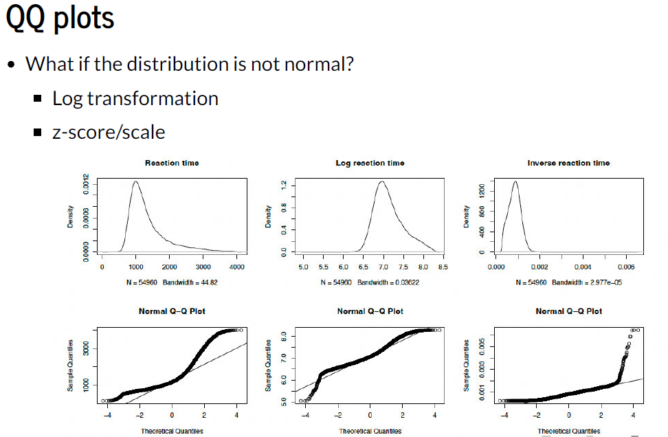
- Skewed distribution
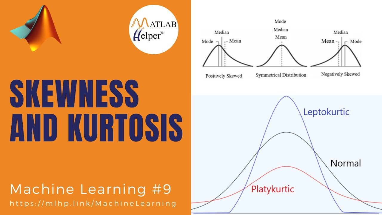
- Positively skewed: tail 指向更大的值
- Negatively skewed: tail 指向更小的值
- Kurtosis distribution
- Leptokurtic: positive kurtosis (heavy-tailed 重尾)
- Platykurtic: negative kurtosis (light-tailed 轻尾)
1.7.2. The center of a distribution
1.7.2.1. The mode (P22)
- 优点:容易找出来,看 frequency plot 中最高的对应的 x 值就是 mode 众数
- 缺点:一个数据集中可能有很多个众数(bimodal, multimodal),不易于知晓数据的分布
1.7.2.2. The median
- 优点:relatively unaffected by extreme scores at either end of the distribution (also relatively unaffected by skewed distributions)
- 可以用于 3 类数据中
- Ordinal
- Interval
- Ratio
- 可以用于 3 类数据中
- 缺点:不能用于 nominal data, 因为 nominal data 没有数字顺序
1.7.2.3. The mean
- 优点:mean 是用上了数据集中每一个数据点所求得的,所以 it is stable in different samples
- 缺点:
- Is affected by skewed distributions
- 只能用于 interval or ratio data
1.7.3. The dispersion in a distribution
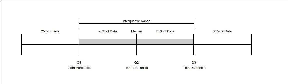
- The median = second quartile
- Q1 也叫做 lower quartile (值较低的那一半的中位数)
- Q3 也叫做 upper quartile (值较高的那一半的中位数)
1.7.4. Using a frequency distribution to go beyond the data
- Z-score
- s 是标准差,见 #SD VS SE
- 我们从数据跨出去的第一步就是,可以计算某一个值出现的概率,即用 z-score
- 一些 z-score 的值是很重要的,因为这些值 cut off certain important percentages of the distribution
| z-score | probability |
|---|---|
| ±1.96 之间 | 95% |
| ±2.58 之间 | 99% |
| ±3.29 之间 | 99.9% |
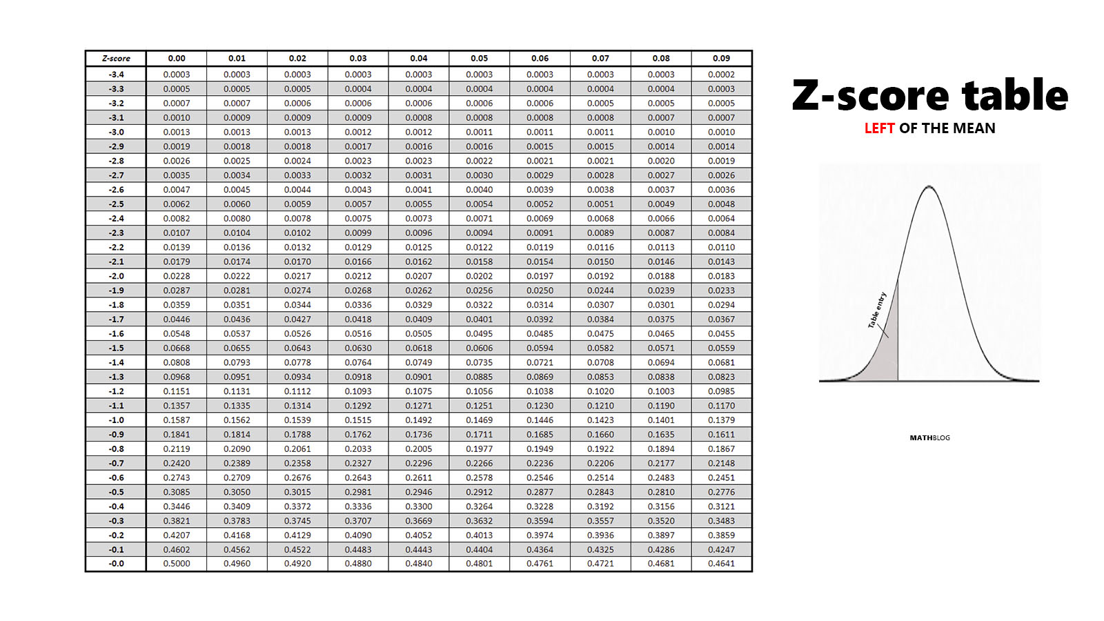
- 怎么看这个表?(以 z=-1.96 为例)
- 纵向找到-1.9, 定位这一行
- 横向找到 0.06, 定位这一列
- 所交叉的单元格就是 z=-1.96 在正态分布图上左边阴影部分的发生概率,即 0.025 (2.5%)
1.7.5. Fitting statistical model to the data
- H1 备择假设:所立的假设/预期效应会出现
- H0 原假设:效应不会出现
- 使用 H0 的原因是:我们不能直接"证实"H1,但我们可以拒绝 H0
- but 尽管能拒绝 H0 ,也不能说接受 accept H1,只能说 support H1
- 使用 H0 的原因是:我们不能直接"证实"H1,但我们可以拒绝 H0
- 有向/无向假设 directional/non-directional hypothesis
- E.g., 有向:读者的统计学知识会增加
无向:读者的统计学知识会变化
- E.g., 有向:读者的统计学知识会增加
SD VS SE
-
标准差 (SD)
- 定义:标准差衡量的是数据集中每个数据点与其均值之间的离散程度。它反映了数据的变异性或分散程度。
- 计算公式:对于样本数据,标准差的计算公式为
- 其中,xi 是每个数据点,
是样本均值,N 是样本数量。
- 其中,xi 是每个数据点,
- 用途:标准差用于描述数据集的总体分布情况,是衡量数据集内部变异的基本指标。
-
标准误 (SE)
- 定义:标准误是样本均值的标准差,衡量的是不同样本均值之间的变异程度,反映样本均值对总体均值的估计准确性。标准误越小,样本均值越接近总体均值。
- 计算公式:标准误通常通过样本的标准差计算,公式为:
其中,SD 是样本标准差,N 是样本大小。 - 用途:标准误用于估计样本均值与总体均值的误差,通常用于构建置信区间和进行假设检验。
-
联系
- 数学关系:标准误与标准差之间的关系通过样本大小 N体现。标准误等于标准差除以样本量的平方根,即这意味着在样本量一定的情况下,样本数据的变异性越大(即标准差越大),样本均值的标准误也越大。
- 用途不同:标准差描述数据本身的分散程度,而标准误描述的是样本均值作为总体均值估计值的可靠性。
总结来说,标准差衡量数据本身的变异性,而标准误衡量样本均值对总体均值的估计精度。随着样本量增加,标准误会减小,表示估计的准确性提高。
C2. Everything about statistics
2.2. Building statistical models (P34)
- Fit: 拟合度;the degree to which a statistical model represents the data that are collected
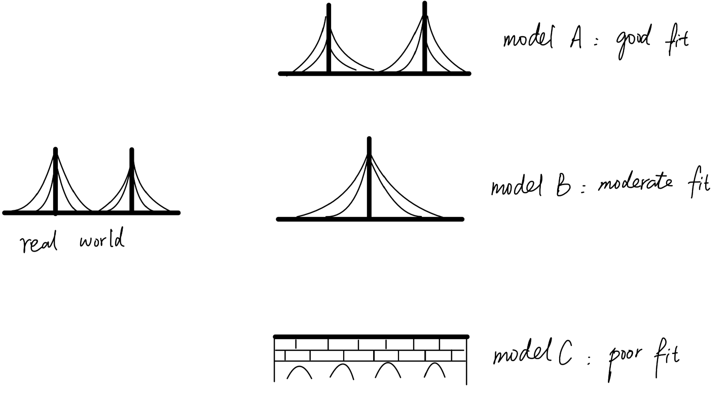
- 以建造桥梁为例,我们实际的桥是左边这样,我根据收集的数据建模出来三个模型 ABC,A 是最能拟合实际桥的模型,所以是 good fit
2.4. Simple statistical models (P36)
2.4.1. The mean: a very simple stats model
- Mean value: 是一个 hypothetical 假设意义上的 model
- Is a model created to summarize our data
- 符号:
表示 population mean 表示 sample mean
2.4.2. Assessing the fit of the mean: sums of squares 平方和, variance 方差, SD 标准差
- 以构建桥梁模型为例 Pasted image 20240928180554.png,how closely the models resembles the real bridge?
- 比较 observed data VS the model
- 此处我们选 the mean 作为 model
- Observed data 有 5 个数据点,不同的数据点与 model (the mean) 存在不同的偏差 deviance, 如何估计 model 的 accuracy?
- 把 5 个 deviance 加起来 = total error
- 若 total error=0, 则 model 是完美 representation of the observed data
- BUT 这肯定不符合事情,因为不同的观测值与 the mean 之间是有差距的,而且或正或负 → 那么,为了避免 error 的方向(正/负),我们把每个 error 平方,然后再加起来,即误差平方和 SS (sum of squared errors)
- 但是 SS 在 observed data 数据点很多的情况下,会变得很大(毕竟是把值加起来)→ 为了避免这一点,用
得到方差 variance
- 此处的 N-1 是自由度 df #如何理解自由度 df?
- 方差是观测值与 mean 的平均误差
- BUT 方差有个问题是它带平方;如果我们的观测值是人数,那么说"朋友的人数是平方后的 1.3 人"显然 does not make any sense → 为了把平方去掉,我们用标准差 standard deviation (SD or s) #SD VS SE
- SD 才是 measure how well the mean represents the collected data
- SD 越小,mean (即 model)更能反应 observed data 的情况
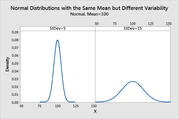
- SD 的重要性还体现在"两个数据集有相同的 mean 值,但 SD 值不同,数据的分布也会不同"
- SD 值小(=5),数据簇拥在一起
- SD 值大(=15),数据分散得比较广
- SD 才是 measure how well the mean represents the collected data
- 但是 SS 在 observed data 数据点很多的情况下,会变得很大(毕竟是把值加起来)→ 为了避免这一点,用
- 比较 observed data VS the model
如何理解自由度 df?
- 假设你是一个足球队的教练,你要安排队员上场后的位置,一个足球队需要 11 个人上场。当第一个候选人来了,他有 11 个位置可以选;第二个人来了,有 10 个位置可选……,第 11 个人来了,就没有选择了,因为只剩下一个位置。
- 所以对前 10 个人来说,他们都有选择位置的自由度,而最后一个人没有自由,这就是自由度(df = N-1)的含义。
- 目的:avoid the introduced bias
2.4.3. Expressing the mean as a model (P40)
- 如何表达 the mean as a model?
- outcomei = (model) + errori
- 当 model 加上个 error 值后,可以 predict observed data
- 我们现在的 model 是 the mean,则
- outcomei =
+ εi - 比如,讲师 A 有 1 个朋友,但所有讲师的朋友均值=2.6,则
- 1=2.6+ε讲师 A
- ε=-1.6
- 那这个 model 与观测值的拟合程度 fit 如何呢?
- 我们用 deviation = SS 误差平方和来求
- outcomei =
2.5. Going beyond the data
- 我们需要 say something general about the world
- Our model is a good fit to the sample? 我们建的模型能拟合已有的样本数据吗?
- Our model is a good fit to the population from which the sample came? 我们建的模型能拟合样本所来自的群体吗?
- Large sample 是指多大?
- N≥30
2.5.1. The standard error (SE) 标准误
- 指标:how well a sample can represent the population
- 标准误 (SE) 是样本均值的标准差 s of sample means
- 若标准误的值大,则不同 sample means 之间的变异大,那么不能用所收集的 sample 来 represent population
- 反之,则可以用所收集的 sample mean 来代表 population
2.5.2. Confidence intervals 置信区间
2.5.2.1. Calculating CI
- 以上我们知道了 SE 可以用来看 sample means 之间的变异程度
- 另一个方法是:计算边界 boundaries,求得我们认为的 mean 的 true value 会 fall in 的区间(即 population value OR real world 所在的区间),这个区间就是置信区间
- 这个区间也可以评估 sample mean 能否反映 population mean 的准确度
- 95%置信区间是什么意思?
- 我们收集了 100 个 samples, 我们所构建的 100 个 confidence intervals 中,有 95 个能 contain the true value of the population mean
- 那如何确定 95%的置信区间的边界值(limits)呢?
- 之前提到过 z=±1.96 很重要,因为在-1.96~1.96 之间的部分就意味着 95%的概率 Pasted image 20240928162432.png
- 但 z=±1.96 是在 mean=0, SD=1 的正态分布情况下才能去查表;而我们的 sample 不是这个配置,就需要转化我们的 sample 为 mean=0, SD=1 的配置
- 把±1.96 放到 z 的位置,可得到
- lower boundary:
Upper boundary: - BUT 实际上我们不用 SD, 而是用 SE 来算 lower/upper boundaries; 因为 SD 是用来看 observed values variability within the sample, 而 SE 是用来看 sample means 之间的 variability
- 所以 lower boundary:
Upper boundary:
- lower boundary:
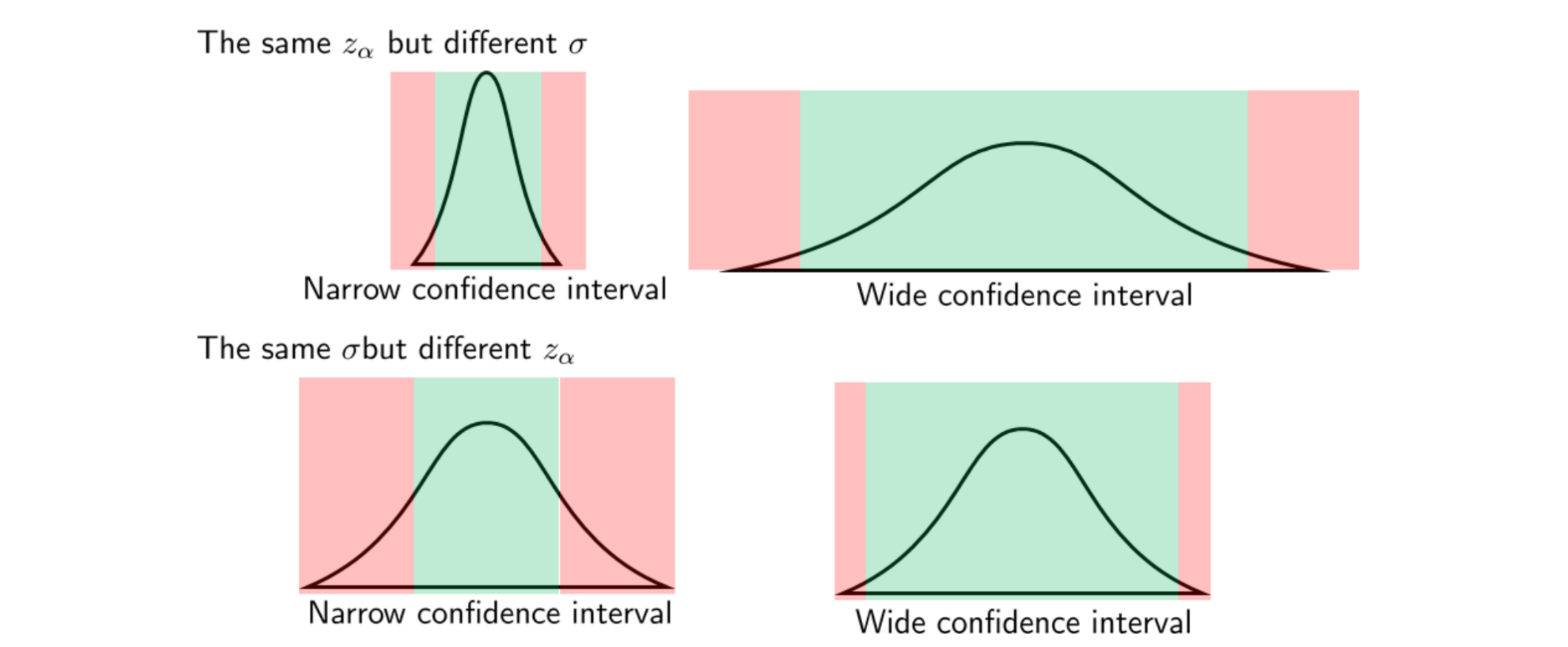
- 可见,mean 是一直在置信区间的 center,如果置信区间窄,那么 sample mean 更能 represent population mean;而如果置信区间宽,那么 sample mean 就不太能代表 population mean
- 置信区间的宽窄,一种情况是如 Pasted image 20240928212707.png 的分布,即也就是下图中的 z-score 相同,但
(即标准差 s)不同 - 左图更能 represent population mean
- 另一种情况是
相同,但 z-score 不同 - 左图更能 represent population mean
- 左图更能 represent population mean
- 置信区间的宽窄,一种情况是如 Pasted image 20240928212707.png 的分布,即也就是下图中的 z-score 相同,但
2.5.2.2. Calculating other confidence intervals
- 如果我们所设的 CI 不是 95%,而是 99%(p=99%), 那此时的 lower/upper boundary 怎么算呢?
- Lower boundary:
- Upper boundary:
- p = 99%, 则对于
(去查表) 的 z-score 为 2.58,就不再是 CI=95%时的 1.96 了
- Lower boundary:
- 但是 CI 的计算要考虑 sample size 的大小,若 n >= 30, 是用 z-score 来算 CI;
若 n<30, 是用 t-score 来算 CI, 这时要用上 df #如何理解自由度 df?
For small sample size
We’re interested to know how many followers people have with on Instagram. We collect a sample of 11 individuals and then calculate the mean and sd. We find that the mean is 96.64 and the standard deviation is 61.27.
a. Calculate a 95% confidence interval for this mean.
Since the sample size is 11, less than 30, we need to use the t-score to calculate the CI
# input data
follower_mean <- 96.64       # Sample mean
follower_sd <- 61.27         # Sample standard deviation
n <- 11                 # Sample size
confidence_level <- 0.95  # 95% confidence level

# Step 1: Calculate the degrees of freedom
df <- n - 1

# Step 2: Get the critical t-score
t_score <- qt(1 - (1 - confidence_level) / 2, df) # that returns the quantile (or critical value) from the t-distribution for a specified probability and degrees of freedom.

# Step 3: Calculate the standard error
standard_error <- follower_sd / sqrt(n)

# Step 4: Calculate the margin of error
margin_of_error <- t_score * standard_error

# Step 5: Calculate the confidence interval
lower_bound <- follower_mean - margin_of_error
upper_bound <- follower_mean + margin_of_error

# Display the results
cat("Sample Mean:", follower_mean, "\n")
cat("T-score for", confidence_level * 100, "% confidence level with", df, "df:", round(t_score, 3), "\n")
cat("Margin of Error:", round(margin_of_error, 3), "\n")
cat("Confidence Interval: [", round(lower_bound, 3), ", ", round(upper_bound, 3), "]\n")
- Confidence Interval: [55.478, 137.802]
For large sample size
b. We collect new data and now we have 56 subject total. Recalculate the confidence interval.
Now the sample size is over 30, we need to use z-score to calculate the CI
# Step 1: Calculate sample statistics
follower2_mean <- 96.64  # Sample mean
follower2_mean
follower2_sd <- 61.27                      # Population standard deviation (known)
follower2_sd
n <- 56          # Sample size
n

# Step 2: Set confidence level and find the z-score
confidence_level <- 0.95          # 95% confidence level
alpha <- 1 - confidence_level     # Significance level (0.05)
z_score <- qnorm(1 - alpha / 2)   # Z-score for 95% confidence. qnorm() returns the quantile (or critical value) of the normal distribution for a given cumulative probability. its like feeding it qnorm(0.975)
z_score

# Step 3: Calculate the standard error
standard_error <- follower2_sd / sqrt(n)  # Standard Error

# Step 4: Calculate the margin of error and confidence interval
margin_of_error <- z_score * standard_error
lower_bound <- follower2_mean - margin_of_error
upper_bound <- follower2_mean + margin_of_error

# Display the results
cat("Sample Mean:", round(follower2_mean, 2), "\n")
cat("Z-score for", confidence_level * 100, "% confidence level:", round(z_score, 2), "\n")
cat("Margin of Error:", round(margin_of_error, 2), "\n")
cat("Confidence Interval: [", round(lower_bound, 2), ",", round(upper_bound, 2), "]\n")
- Confidence Interval: [80.59, 112.69]
2.5.2.4. Showing confidence intervals visually
- 画图时,用 error bar 显示出 CIs
- 表示 95%置信区间 of the mean
- 这样一来就可以看出不同 sample means 是否来自 the same population
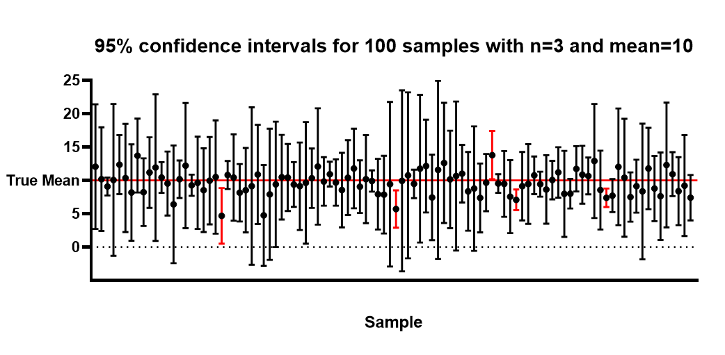
- 从这张图我们就能看到,红色线条代表的 samples 由于没有把 mean=10 囊括在自己的 error bar 范围内,可以推测,红色线条的 samples 与黑色线条的 samples 不是来自同一个 population
- → 很可能意味着我们的 experimental manipulation has induced a difference between the samples.
2.6. Using statistical models to test research questions
- 为什么要用 95%的 confidence interval?
- Fisher 指出:只有当我们有 95%的信心 confidence 确定 a hypothesis is genuine (即 not a chance finding)时,我们才能接受这个发现是 true/genuine
2.6.1. Test statistics
- 通过 fit statistical model to data that represent the hypothesis we want to test
&
Use probability to see whether scores are likely to happen by chance
- Probability: the likelihood of a particular outcome given a set of possible outcomes
- 概率是可以加起来的,只要 the outcomes of interest are independent and mutually exclusive 独立且互斥
- 如一颗色子抛一次,出 1 点或2 点或3 点朝上的概率为:
- 那么,结合这两个操作,我们可以 test 我们的 stats models (同时也是 hypothesis) 是否 significantly fit the data that we collected.
- 一个好办法来算 whether the model fits the data (即我们的 hypothesis 是否 is a good explanation of the data),就是算 test statistic
- Test-statistic 可以写成 t, F, x2
-
- 这里的 test statistic 就是
的 ratio - Systematic variance: 系统变异,可以由 the model that we have fitted to the data 解释的变异
- unsystematic variance: 非系统变异,不可由我们拟合到 data 的 model 解释的变异 #1.6.2.2. Two types of variation
- 若我们的 model 能很好地解释很多的 variance, 即
的话,则
- 一个好办法来算 whether the model fits the data (即我们的 hypothesis 是否 is a good explanation of the data),就是算 test statistic
- 如果一个 statistical model that we fit to the data 能反映 the hypothesis that we set out to test, 那么所求出来的 significant test statistic 就能告诉我们:
- 这个 model 绝对不可能反映不出 real world 的 population (即这个 model 绝对不可能反映出 null hypothesis is true)
- → 此时,我们可以 reject our null hypothesis, and gain confidence that the alternative hypothesis is true. 【但不能说 we accept H1, 见 #1.7.5. Fitting statistical model to the data,我们只能说 support H1 】
- 其实也有另一个方法,不需要拒绝 H0 , Bayesian statistics, 因为 Bayesian 是认为构建一个 Null hypothesis is stupid
Jane superbrain 2.6 (P54)
- 从一个 significant test statistic 中我们 CAN & CANNOT 得到的信息
| CAN | CANNOT | |
|---|---|---|
| 1 | "there is a significant effect of ..." | "the effect is important" 因为,very small and unimportant effects can turn out to be statistically significant just because huge numbers of people have been used 只要招的人够多,再小、再不重要的效应都可以变成统计学意义上的“显著”效应 |
| 2 | 若算出来的 test statistic occurring by chance 的概率 > 0.05, 我们可以 reject H1 | "the H0 is true" 因为 H0 的含义是:there is no effect in the population;就算是 test statistic > 0.05, 也只能说明 H0 is true 的概率很大,而不是说 H0 就是true |
| 3 | 若算出来的 test statistic occurring by chance 的概率 < 0.05, 我们可以 reject H0 | "the H0 is false" 同理,只能说明 H0 is false 的概率更大,但不能说明 H0 就是false |
2.6.2. One-and two-tailed tests
-
One-tailed test: 用于 test 有向假设
-
Two-tailed test: 用于 test 无向假设
-
例子:
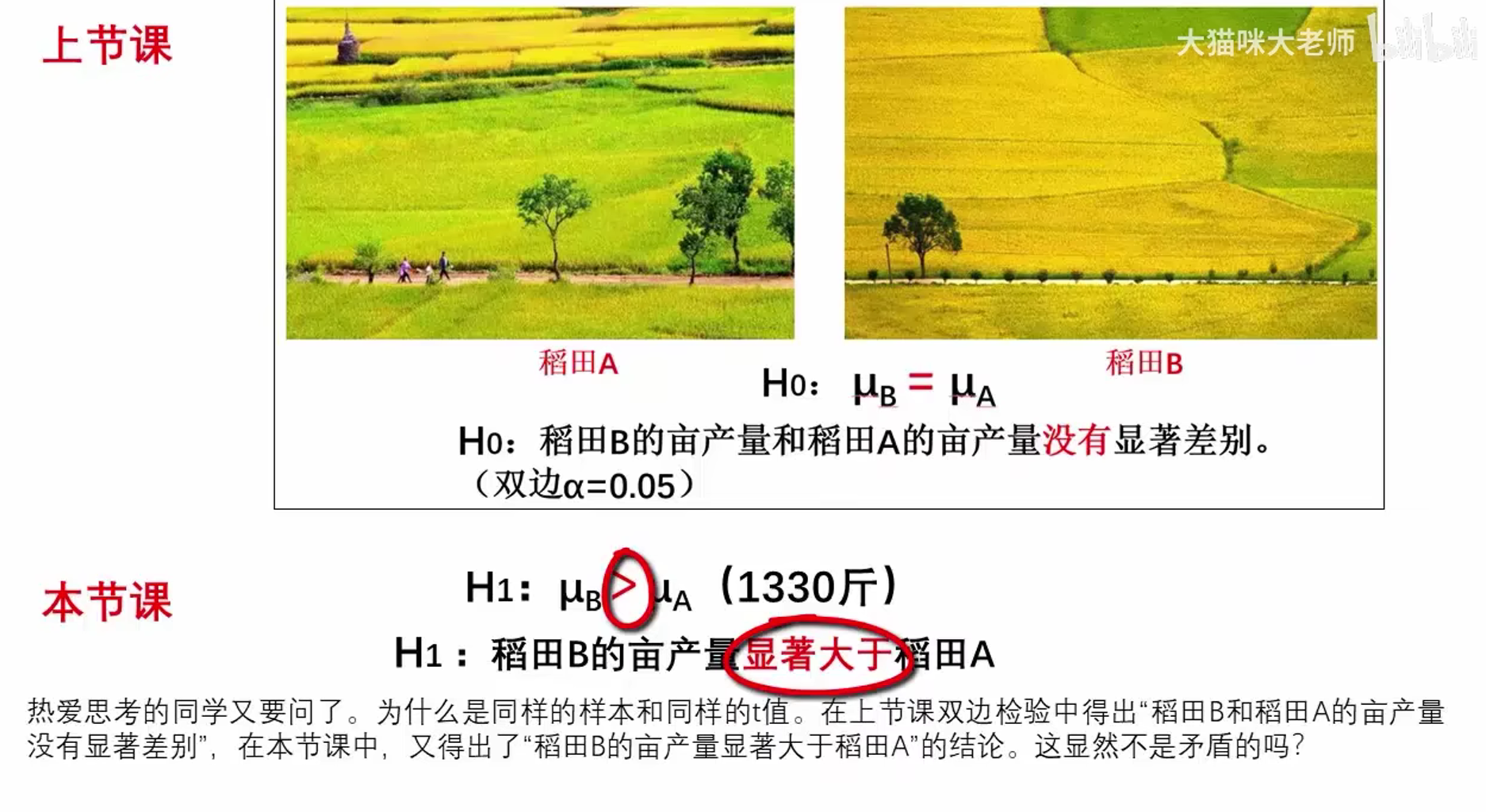
- H0: 读这本书的人与没读的人想杀掉作者的企图没有差别
- H1: 读这本书的人想杀作者的企图>没读这本书的人
Mean1-mean2>0 (positive relationship) - H1: 读这本书的人想杀作者的企图<没读这本书的人
Mean1-mean2<0 (negative relationship)
-
为什么实际统计检验中用 p=0.01 甚至更小的 p=0.001?
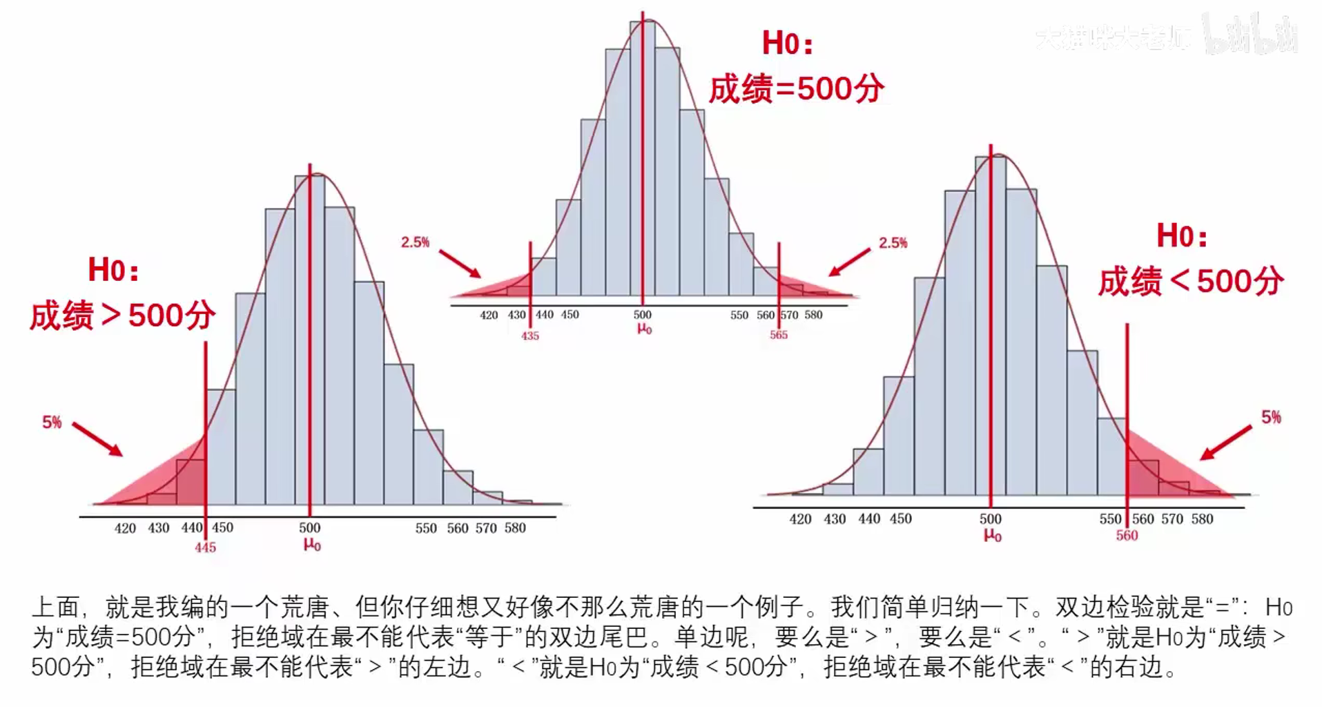
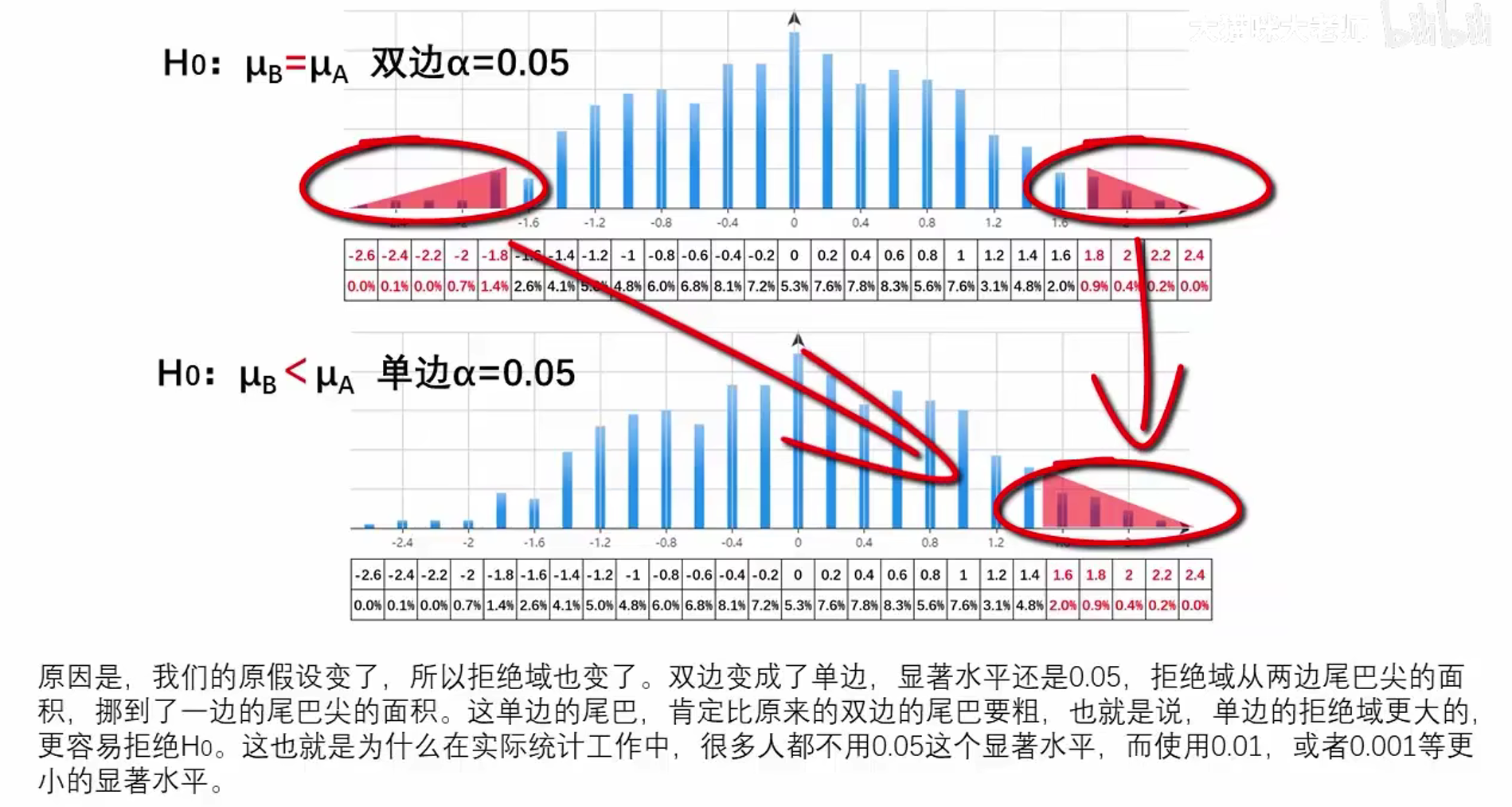
- 单边 VS 双边检验,拥有同样的 p=0.05,可是拒绝域却不同,单边检验的尾巴更粗
- 所有实际的统计检验中很多人用更小的 p 值,以便单边和双边检验的结果不会矛盾 【更多可以看 B 站视频】
url: https://www.bilibili.com/video/BV1oP4y177Qh/?spm_id_from=333.788&vd_source=f1111db8c0296ebbc68186619f534b4f
title: "通俗统计学原理入门7 单边检验 单边假设检验 单边t检验 单尾检验 单侧检验_哔哩哔哩_bilibili"
description: "新年,收获了人生的第一个1000个粉丝。觉得很好玩,完全是无心插柳。本来是带着功利心开始做这个统计学微课视频的,没想到无意中帮助了很多陌生人。感觉冥冥中,印证了“应无所住,而生其心”这句话。当然,这句话也是我对正态分布和中心极限定理的领悟。本学期我也确实上了这门课,见证过同学们“领悟”的那一刻。他们“哦”的那个表情,是不会骗人的。那个瞬间,我是最欣慰的,感觉像度了一个人一样。粉丝留言里,还真有一位, 视频播放量 84689、弹幕量 340、点赞数 2241、投硬币枚数 1722、收藏人数 1773、转发人数 506, 视频作者 陈祥雨大猫咪老师, 作者简介 ,相关视频:SPSS非参数检验视频教程汇总(非常重要,建议收藏!),通俗统计学原理入门12 - 置信区间 Confidence Interval 区间估计 点估计 t临界值 标准误,通俗统计学原理入门10 p值的含义 p value,通俗统计学原理入门6 关键一步 从均值抽样分布到t分布,一招搞定单/双侧检验判断|假设检验|统计学|快速口诀,通俗统计学原理入门8 自由度 单样本t检验自由度,从图上看假设检验里的两类错误以及它们的关系,如何选择统计学方法?T检验、单因素方差分析、秩和检验、卡方检验到底应该选择哪一个?一个视频轻松搞定,通俗统计学原理入门 - t检验 正态分布 显著水平,关于假设检验的一切 - 统计学"
host: www.bilibili.com
image: //i0.hdslb.com/bfs/archive/71af0de10c4d4d71c65398c560994850f0d2f677.jpg@100w_100h_1c.png
- 下图我们可以看到,同样的 p=0.05,可是拒绝域却不同,单边检验的尾巴更粗
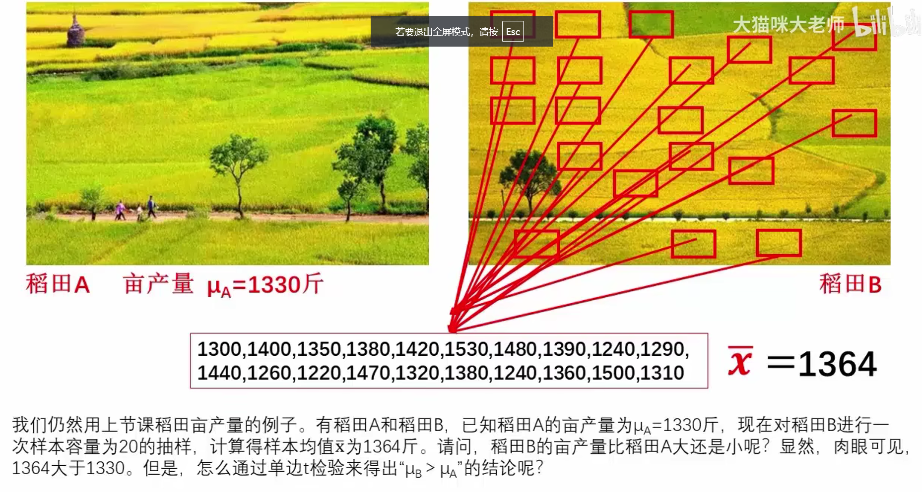
- T 检验;算 t 值
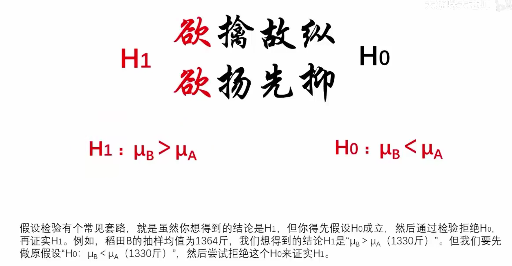
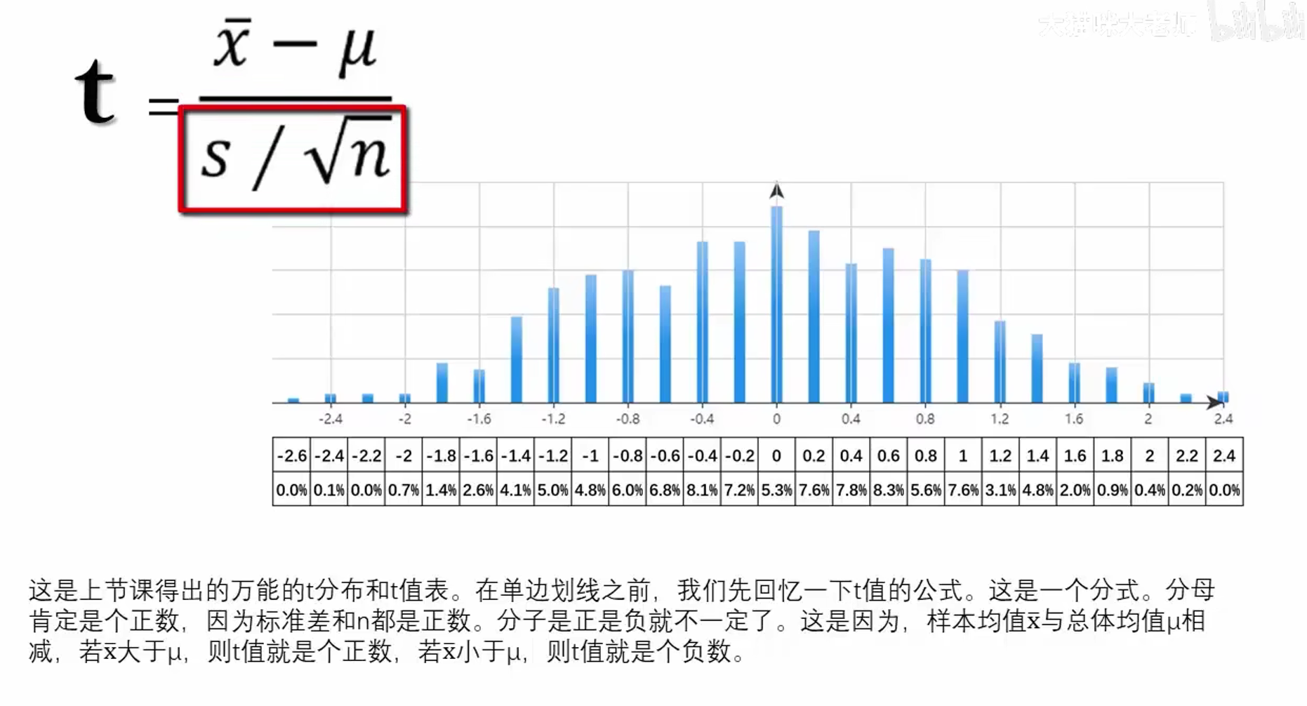
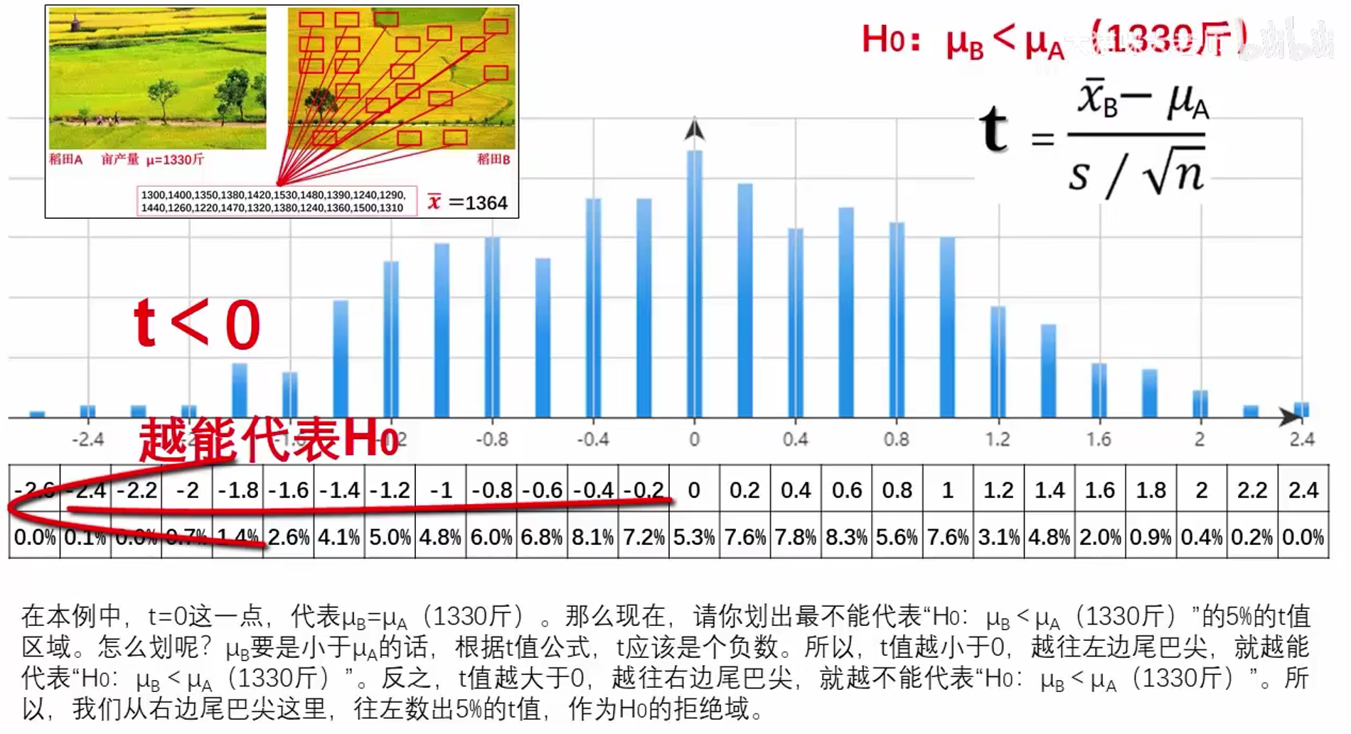
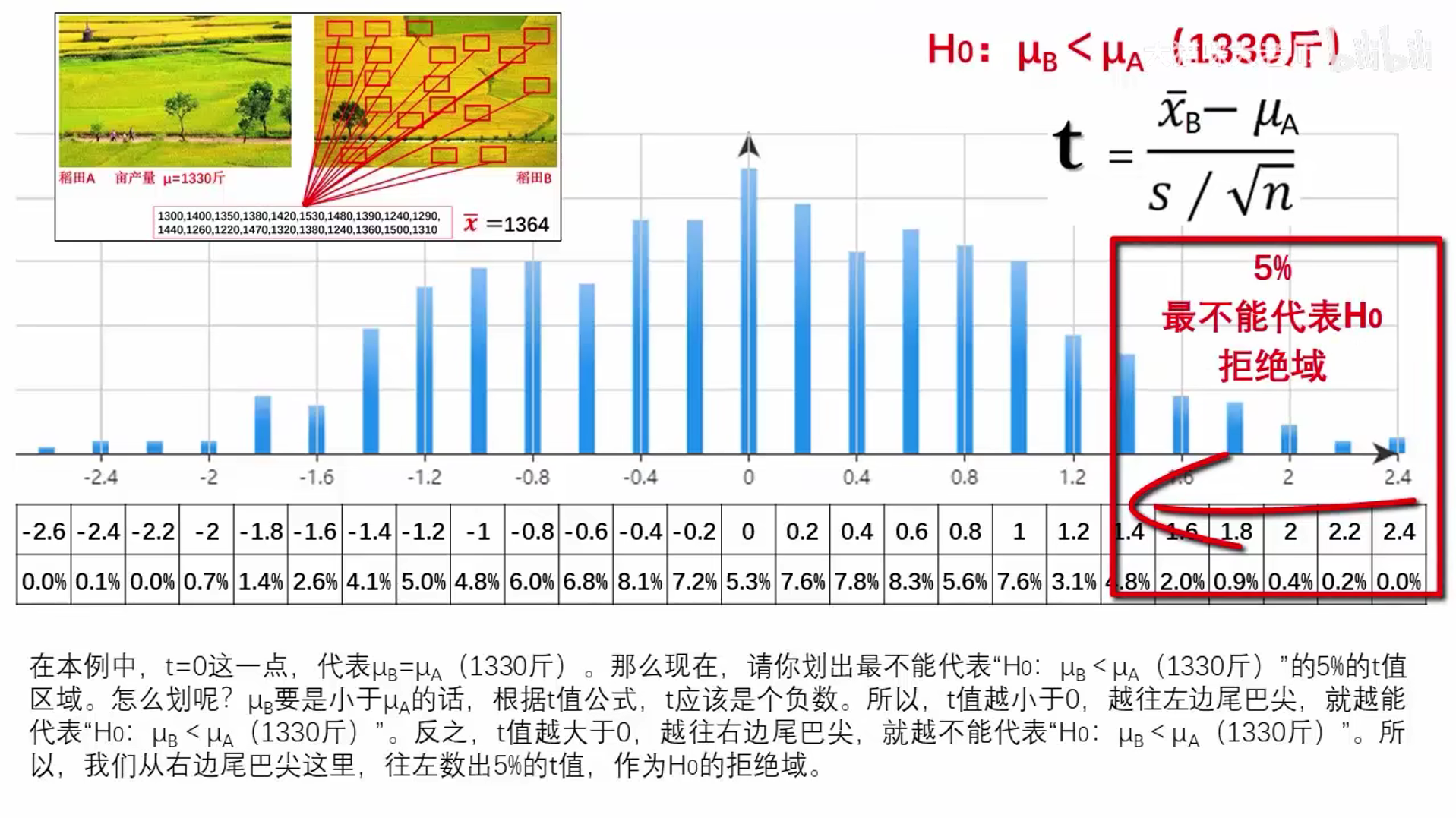
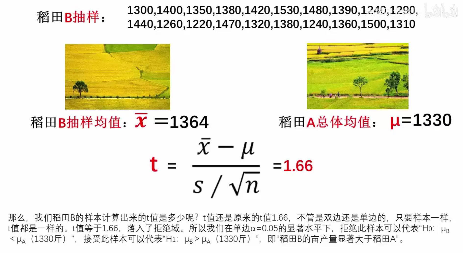
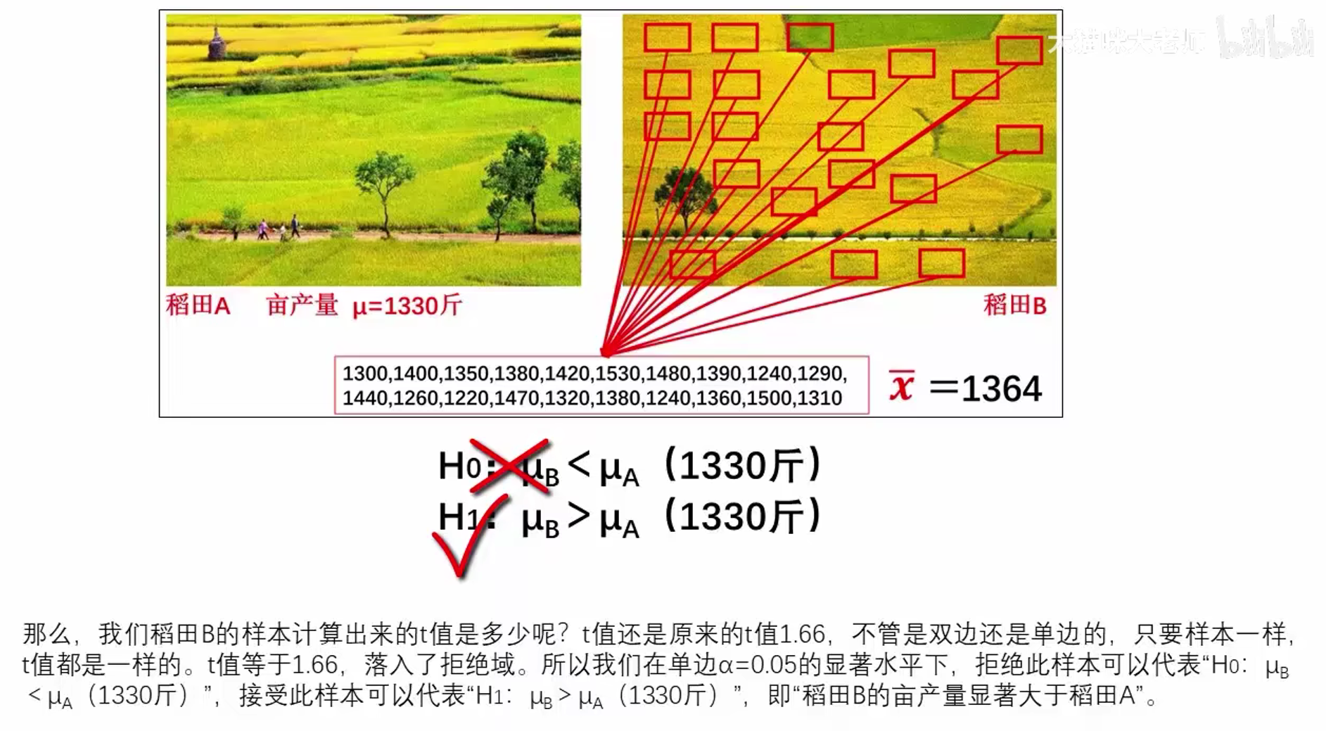
∵原假设从双边变成了单边
2.6.3. Type I & Type II errors
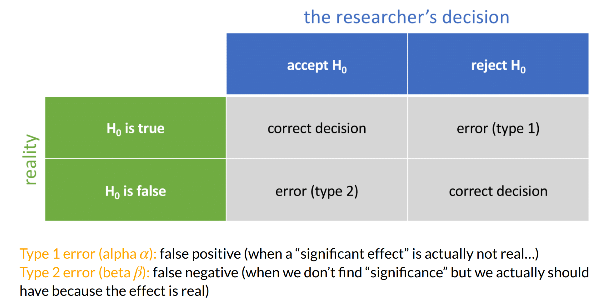
- Type I error: 实际 population 没有这个 effect,但我们却认为有
- 可能发生在:我们重复 data collection 100 次,其中 5 次得到的 test statistic 足够大,让我们以为 population 中也有这个 effect
- The probability of this error: 0.05 (即
-level = p-value) - 如何避免|减少犯错几率?
- Replication,
- Larger sample size,
- More restrictive "significance" level,
- correct for multiple comparisons
- Type II error: 实际 population 有这个 effect,但我们却认为没有
- 可能发生在 obtain a small test statistic 时;因为我们的 samples 之间有其他的 natural variation
- The probability of this error: maximum 0.2 (即
-level = power) -level 的最大可接受值为 20%,意味着 - 若我们从有 effect 的 population 中取出 100 个 samples,里面最多有 20 个 samples detect 不到 effect
- 如何避免?
- Increase sample size,
- Power analysis
| 实际上:被告无罪(Null 为真) | 实际上被告有罪(Null 为假) | |
|---|---|---|
| 判无罪 | ✅ 正确 | ❌ Type II Error(漏判) |
| 判有罪 | ❌ Type I Error(误判) | ✅ 正确 |
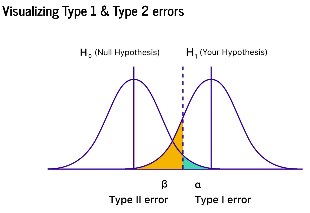
- Type I error (
-level) 祖母绿部分 - Type II error (
- level) 橙色部分
2.6.4. Effect size
- 仅凭 test statistic is significant 并不能意味着 the effect it measures is meaningful or important
- → 那就需要用 effect size 来解决这个问题
- Effect size 定义:an objective and (usually) standardized measure of the magnitude of observed effect
- Standardized 标准化的指标就意味着
- We can compare effect sizes across different studies that have measured different variables
Or have used different scales of measurement (如:以 ms 为度量的 effect size 可以跟以心率为度量的 effect size 进行比较)
- We can compare effect sizes across different studies that have measured different variables
- All psychologists report these effect sizes in the results of any published work, 所以写效应量是个好习惯
- Standardized 标准化的指标就意味着
- Measures of effect size
- 作者是推荐用 Pearson's r, 因为其取值范围是 (0,1),0 代表 no effect,1 代表 a perfect effect
- Pearson's r=0.10 (small effect): the effect 能解释 1%的 total variance
- Pearson's r=0.30 (medium effect): the effect 能解释 9%的 total variance
- Pearson's r=0.50 (large effect): the effect 能解释 25%的 total variance
- 注意:r 不是一个 linear scale;若说 r=0.6 是 r=0.3 的两倍,这么说是不对的
- 但 Cohen's d 的优先使用场景是
- When group sizes are very discrepant 组与组的 size 差异太大时,如 A 组 100 人,B 组 50 人,C 组 10 人
- 取值范围是: 无限~0
- Small effect size: d = 0.2
- Medium: d =0.5
- Large: d >= 0.8
- 统计学啊,实际上我们感兴趣的是 the effect size in the population, 但我们又不能 have access to this value, 我们只能用 the effect size in the sample 来 estimate the likely size of the effect in the population
- 拓展:因为 effect size 是个 standardized value,所以可以将研究同一个 question 的不同 studies 的结果放在一起对比,从而 get better estimates of the population effect size, 这就是 meta-analysis
Meta-analysis
-
Meta-analysis 一般都会把结果放到一个 Forest plot 进行呈现,像这样
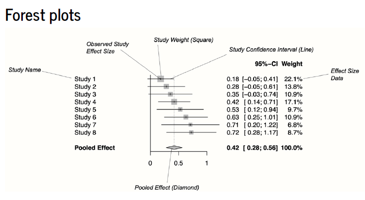
-
更多关于 meta-analysis 的,可以看这个网页 link
2.6.5. Statistical power
- 上面提到的 effect size 其实与其他 3 个 statistical properties 是有关联的 (即知道其中 3 个,就能求出第四个的值),分别是:
- The sample size: the sample effect size is based on
- The probability level: 我们 accept an effect as being statistically significant (即
-level ) - The ability of a test 去 detect an effect of that size (statistical power),即 1-
=0.8 (因为 -level 是我们 fail to detect the effect 的概率)
- 通常,心理学中
- The sample size: 主试肯定知道招了多少人
- The probability level:
-level =0.05 - The ability of a test to detect an effect of that size: 1-
=0.8 - 那么,算出 effect size in a population 就容易了!
- 但更常见的是求我们的 sample size 需要多少人才能达到我们的 statistical power (0.8)?
- 当然可以用上面的已知 3 个,求第四个来算
- 也可以用软件帮我们计算
G*Power,免费nQuery Adviser, 付费- R 包
pwr,免费
C3. The R environment
见 E:/R/dsur/C3R_environment/Chapter 3 The R Environment.R
C4. Exploring Data with Graphs
- 色彩搭配网站 color-hex
url: https://www.color-hex.com/
title: "Color Hex Color Codes"
description: "Color hex is a easy to use tool to get the color codes information including color models (RGB,HSL,HSV and CMYK), css and html color codes."
host: www.color-hex.com
favicon: /favicon.ico
4.2.2. What makes a good graph (7 points)
- Show the data
- Induce the reader to think about the data being presented (rather than how pink it is)
- Avoid distorting the data
- Present many numbers with minimum ink
- Make large data sets coherent
- Encourage the reader to compare different pieces of data
- Reveal data
画图应注意的点
- Never use 3D plots for a graph plotting two variables, ∵it obscures the data, and the 3D effect makes the error bars almost impossible to read
- Never distract the eye from what matters
- Labels should be informative
- Minimum ink to graph is better
4.4. Introducing ggplot2
4.4.1. The anatomy of a plot
-
A graph is made up of a series of layers
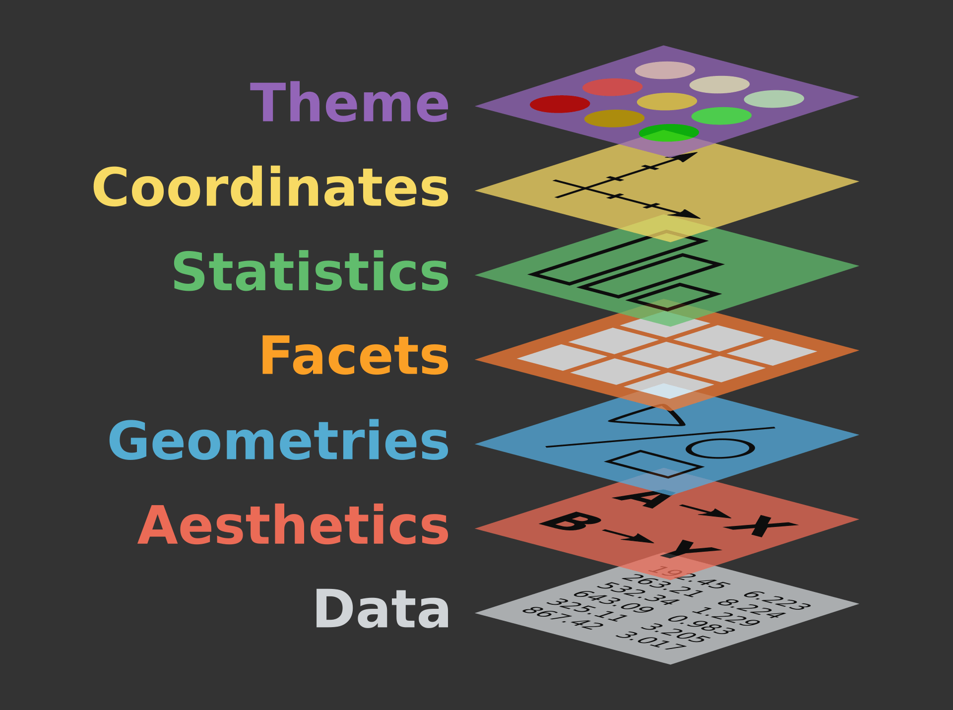
-
Table 4.1 aesthetic properties associated with some commonly used geoms
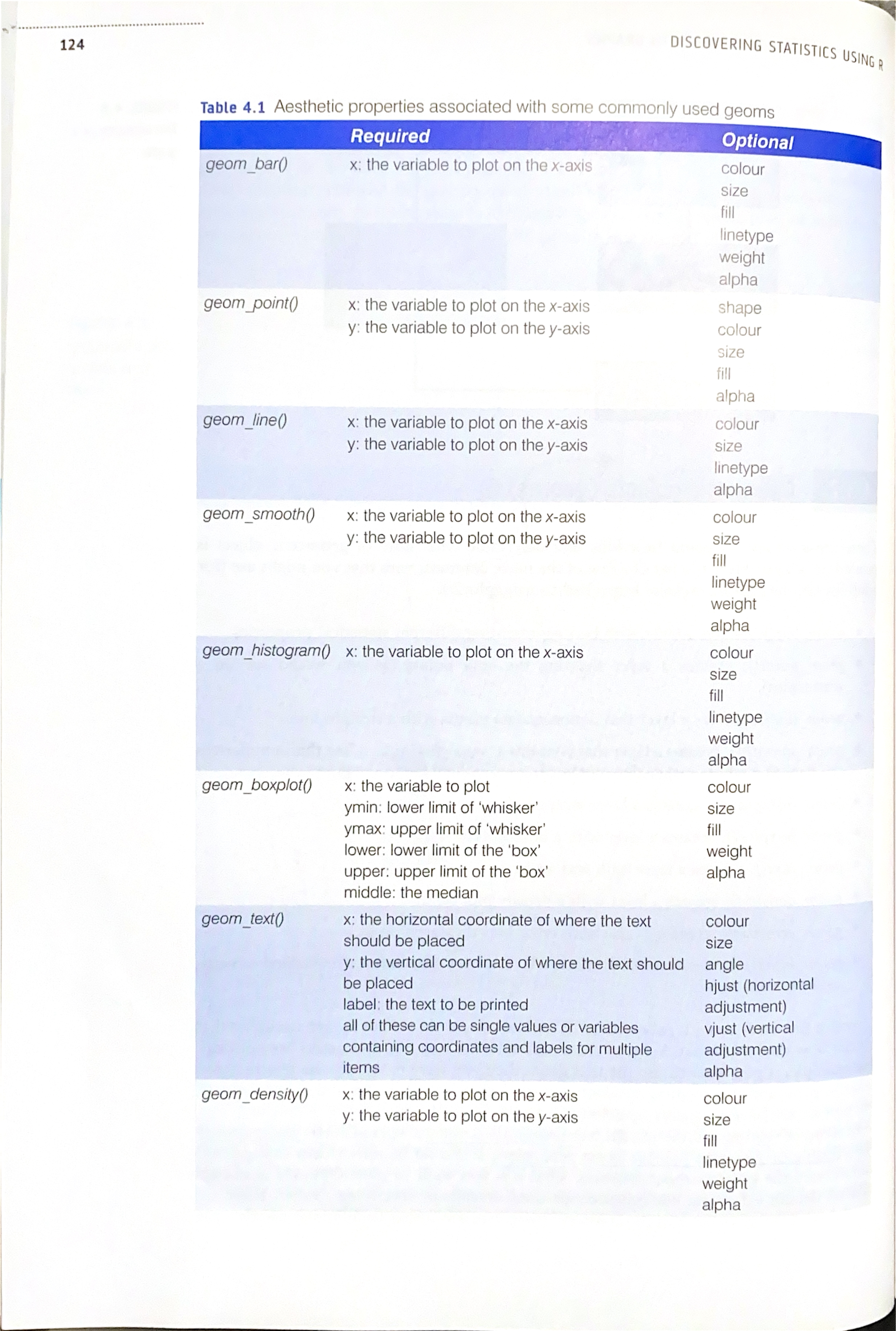
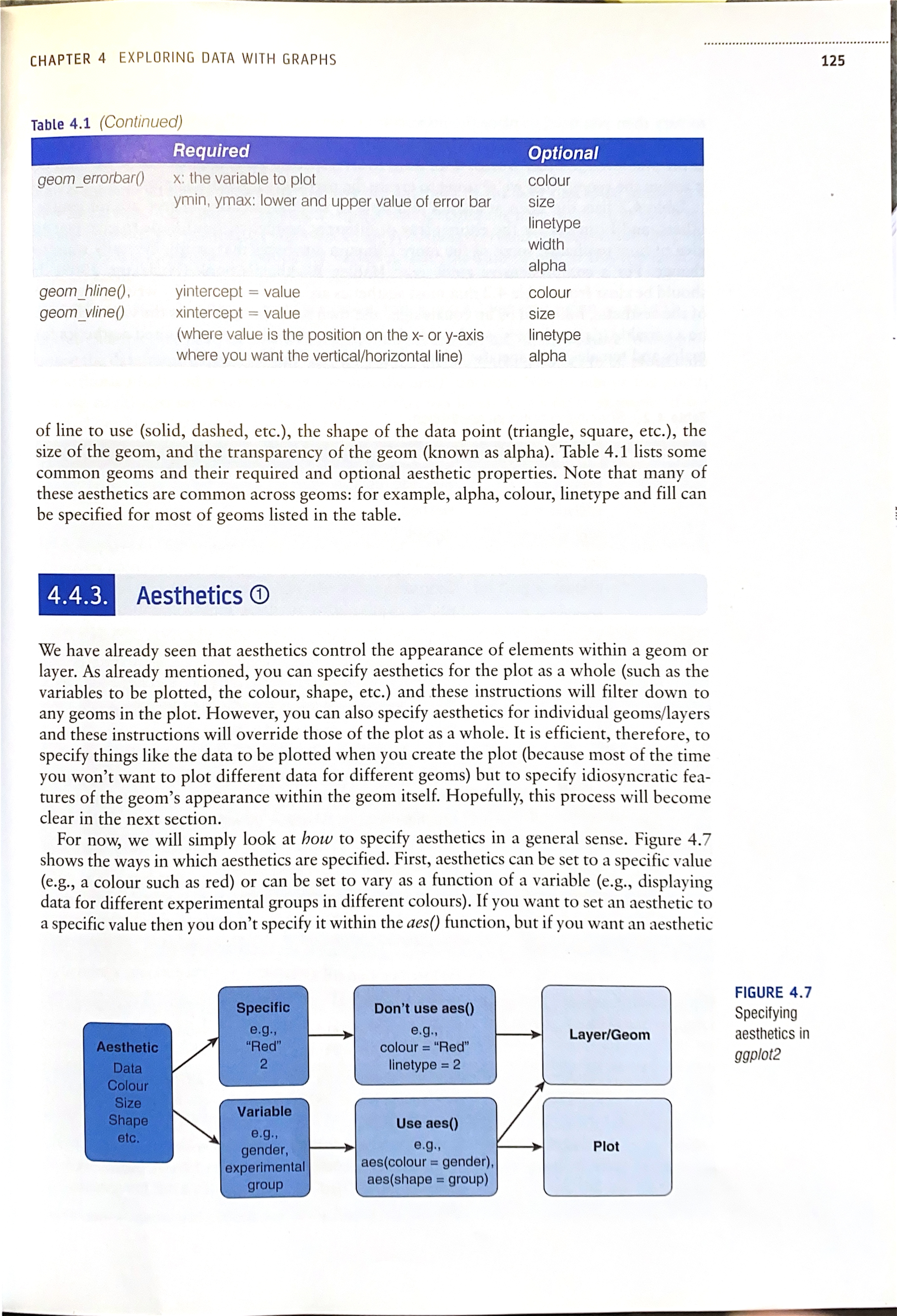
4.4.3. Aesthetics
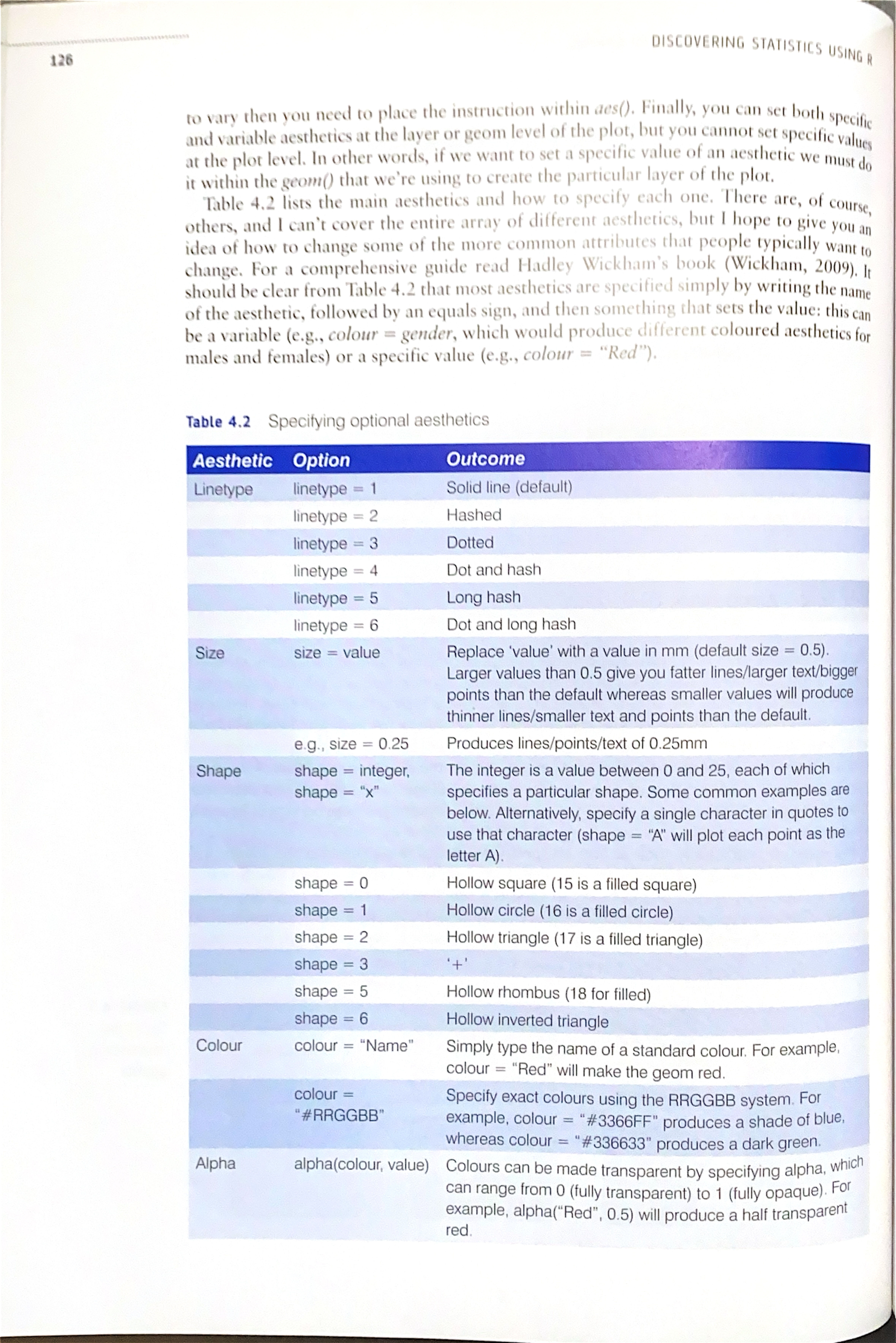
- Table 4.2 specifying optional aesthetics
4.4.5. Stats and geoms
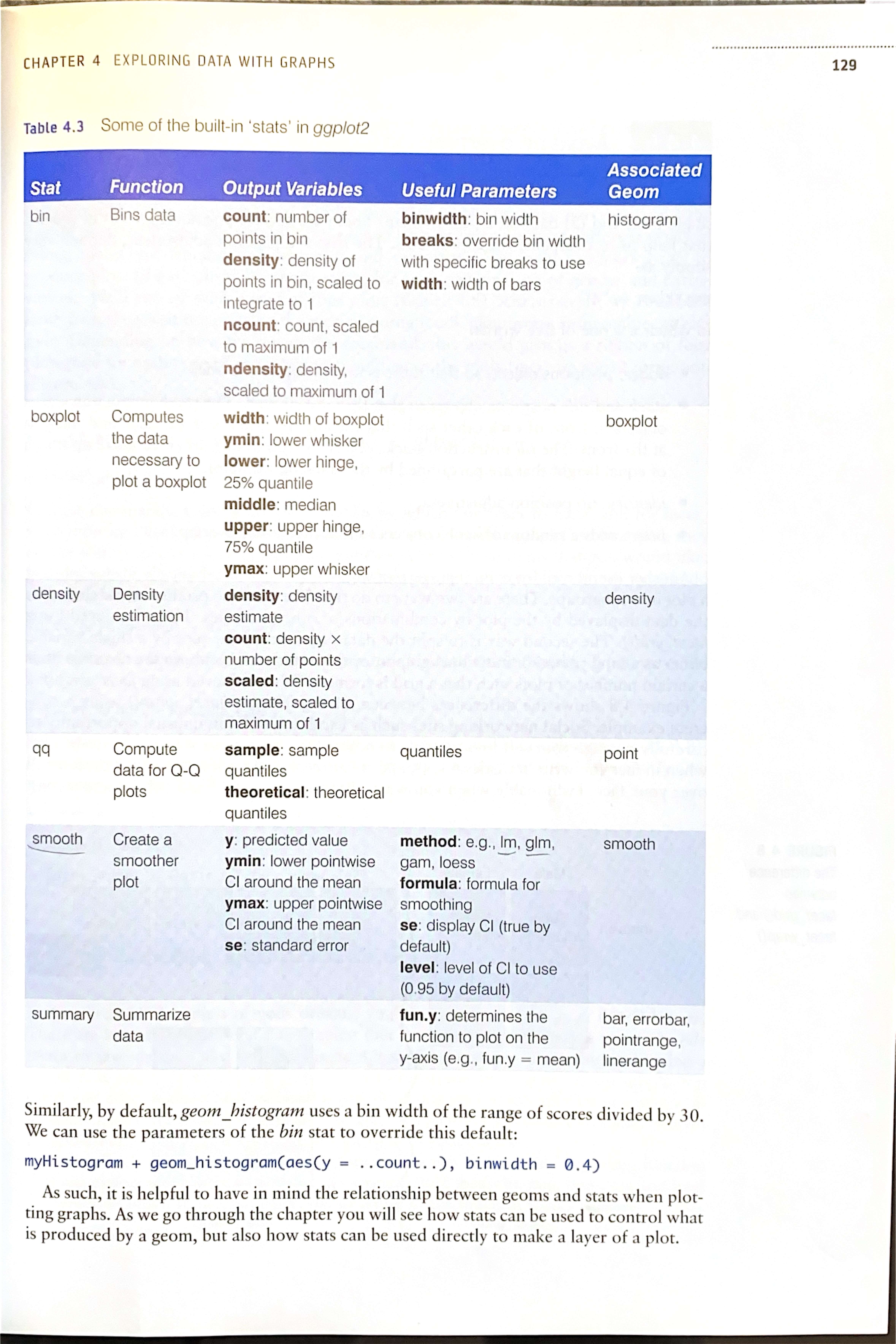
- Table 4.3 some of the built-in 'stats' in ggplot2
4.4.6. Avoiding overplotting
- Faceting: split a plot into subgroups
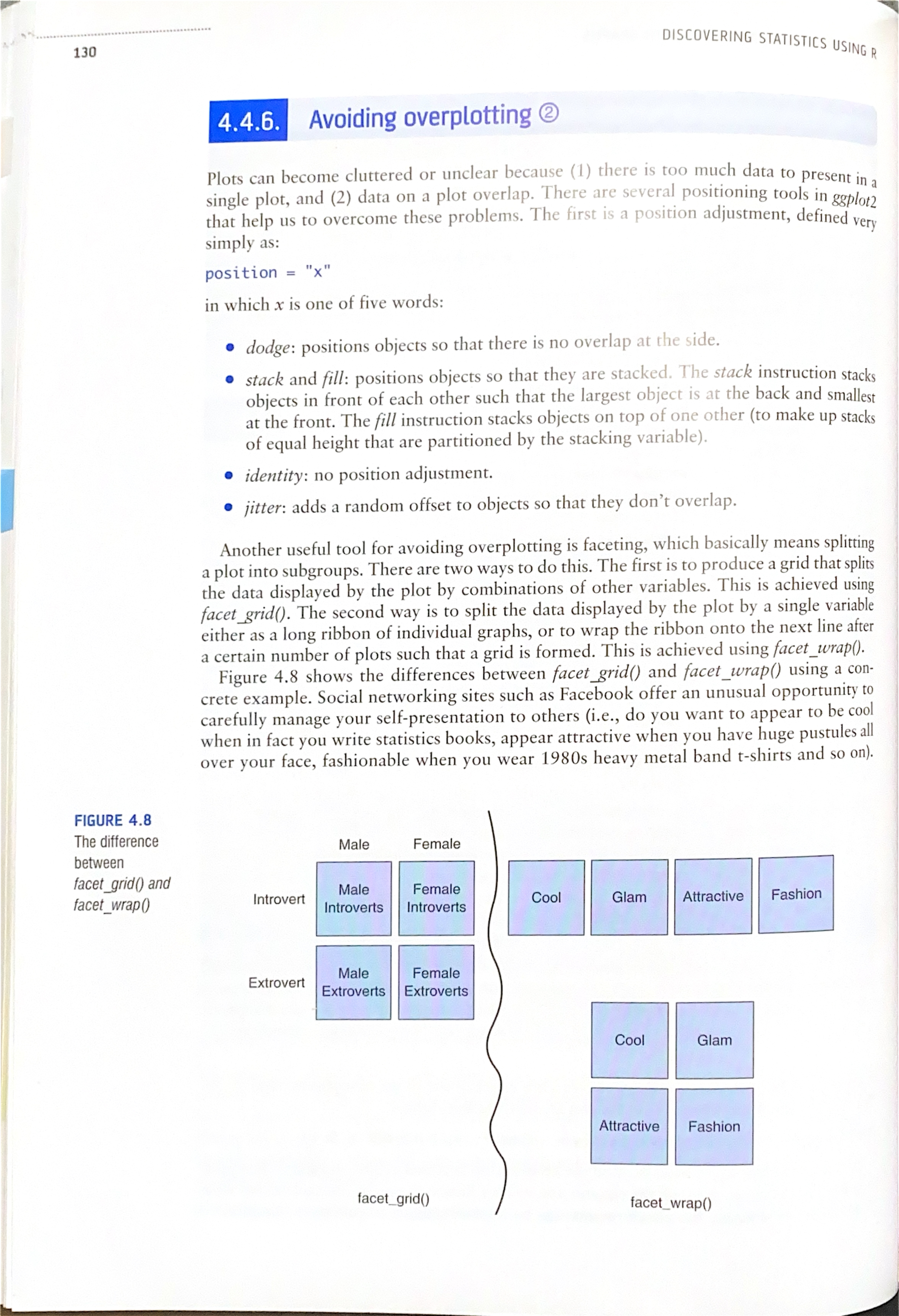
- Facet_grid () 比较适合用于呈现 variables combinations 的结果,如 2
2 的因素设计,就可以用 4 张小图呈现,方便读者进行不同因素间效果的对比 - Facet_wrap () 比较适合用于呈现适用于单因素设计(One-Way Design) 或多水平单因素设计(One-Way Design with Multiple Levels)的结果
- Facet_grid () 比较适合用于呈现 variables combinations 的结果,如 2
- Figure 4.8 the difference between
facet_grid ()andfacet_wrap ()
4.4.7. Saving graphs
ggsave(filename)
# e.g.
ggsave("outlier amazon.png", width = 2, height = 2)
4.4.8. Quick tutorial
#set cran for r code running in obsidian
options(repos = c(CRAN = "https://cran.r-project.org"))

#Set the working directory (you will need to edit this to be the directory where you have stored the data files for this Chapter)

setwd("E:/R/dsur/C4exploring_data_with_graphs")
imageDirectory<-"E:/R/dsur/C4exploring_data_with_graphs/C4_images"

#imageDirectory<-file.path(Sys.getenv("HOME"), "Documents", "Academic", "Books", "Discovering Statistics", "DSU R", "DSU R I", "DSUR I Images")


######A function to make it quick to save graphs in the image directory

saveInImageDirectory<-function(filename){
	imageFile <- file.path(imageDirectory, filename)
	ggsave(imageFile)
}


######Initiate packages

#If you don't have ggplot2 installed then use:
install.packages(c("ggplot2", "plyr"))


#Initiate ggplot2
library(ggplot2)
library(reshape)
library(plyr)
#--------4.4.8.Quick Tutorial----------
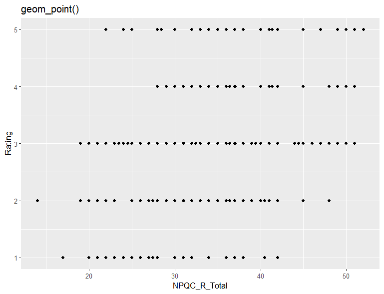
facebookData <- read.delim("FacebookNarcissism.dat.txt",  header = TRUE)

graph <- ggplot(facebookData, aes(x = NPQC_R_Total, y = Rating))
graph +
    geom_point() +
    ggtitle("geom_point()")
graph +
    geom_point(shape = 17) +
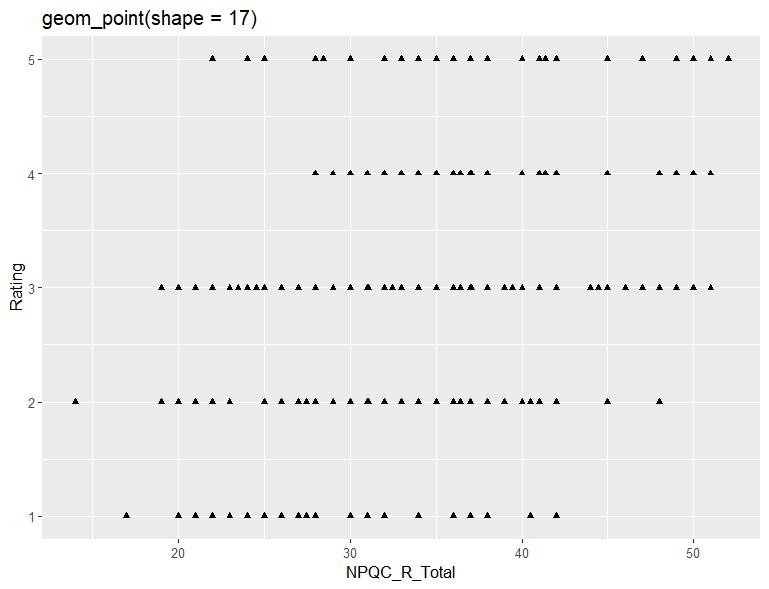
    ggtitle("geom_point(shape = 17)") #shape = 17 is a triangle
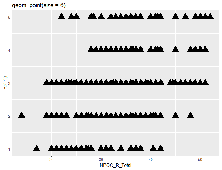
graph +
    geom_point(size = 6, shape = 17) +
    ggtitle("geom_point(size = 6)")
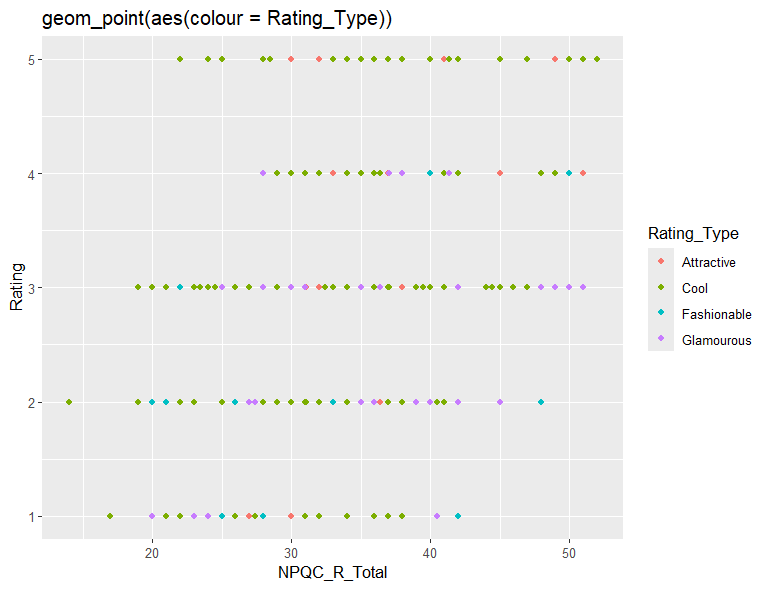
graph +
    geom_point(aes(colour = Rating_Type)) +
    ggtitle("geom_point(aes(colour = Rating_Type))")
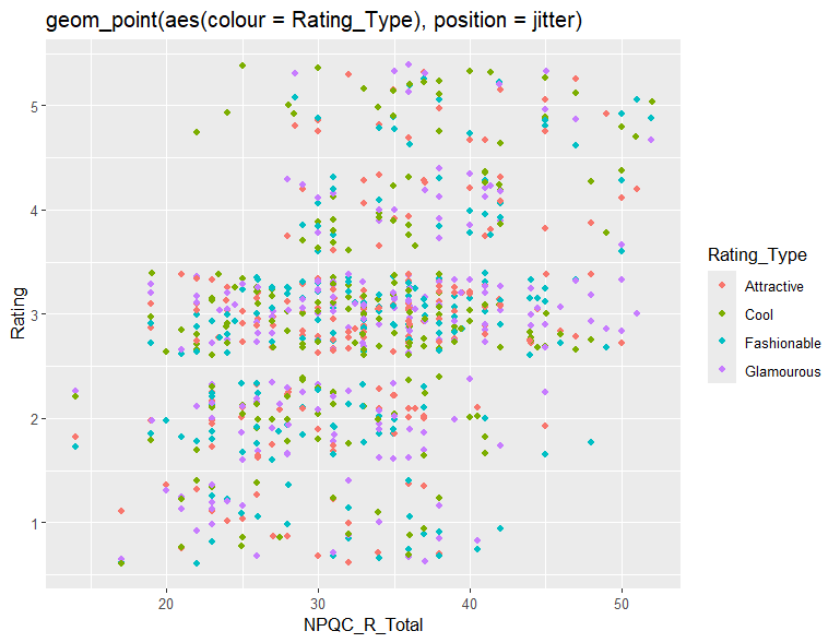
position = "jitter"可以使相同值的数据点不会被覆盖,尤其适用于:同一个被试参与多个测试后,有几个测试的成绩是相同的,但我们想看到这个被试的所有数据点分布
graph +
    geom_point(aes(colour = Rating_Type), position = "jitter") +
    ggtitle("geom_point(aes(colour = Rating_Type), position = jitter)")
graph +
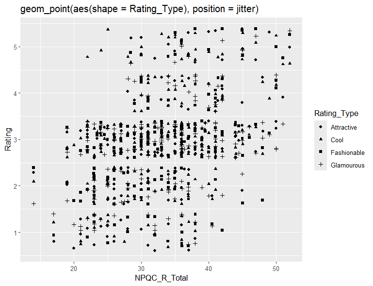
    geom_point(aes(shape = Rating_Type), position = "jitter") +
    ggtitle("geom_point(aes(shape = Rating_Type), position = jitter)")
4.5. Scatterplot
- 散点图适用于 look at the relationships between variables 看变量之间的关系
- 能告诉我们:
- whether there seems to be a relationship between the variables
- What kind of relationship it is
- Whether any cases are markedly different from the others -> to find outliers
4.5.1. Simple scatterplot
- Looking at just two variables
examData <- read.delim("Exam Anxiety.dat.txt",  header = TRUE)
head(examData)
names(examData)
# Simple scatter
scatter <- ggplot(examData, aes(x = Anxiety, y = Exam))
scatter +
    geom_point() +
    labs(x = "Exam Anxiety", y = "Exam Performance %")
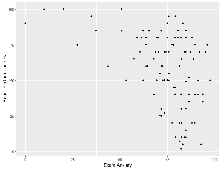
- 从这个散点图中我们可以看到
- 大多数数据分布在 high levels of anxiety 方向
- No obvious outliers
- Low levels of anxiety are almost always associated with high exam performance
- No cases having low anxiety and low exam performance
4.5.2. Adding a funky line
- ggplot2 里面把 regression line 叫做“smoother”,由
geom_smooth()function 实现,可以加上直线或曲线的回归线 - The shaded area around the line is the 95% confidence interval around the line
- Curved line
- Straight line
- Method = "lm"
#Simple scatter with geom_smooth()
scatter <- ggplot(examData, aes(x = Anxiety, y = Exam))
scatter +
    geom_point() +
    geom_smooth() +
    labs(x = "Exam Anxiety", y = "Exam Performance %")
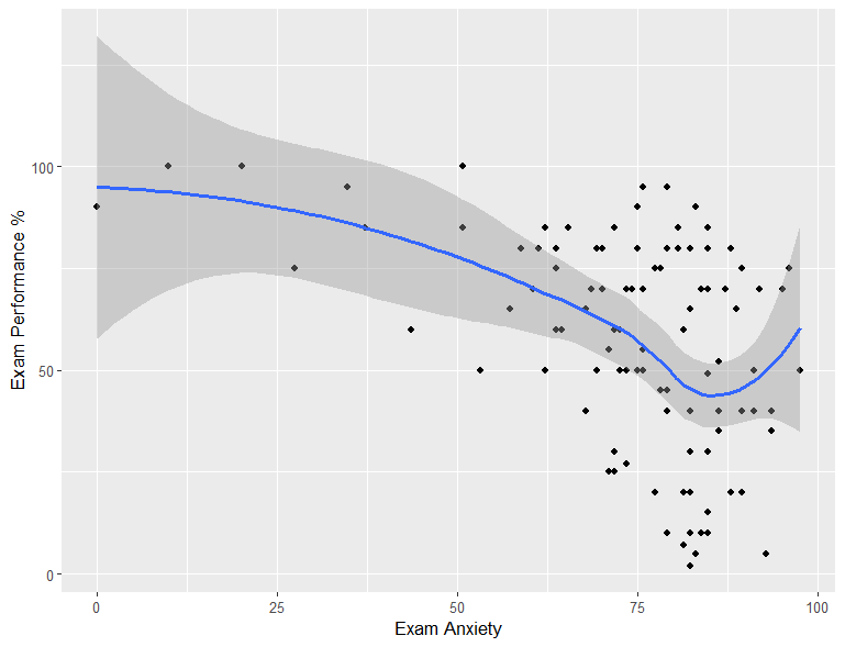
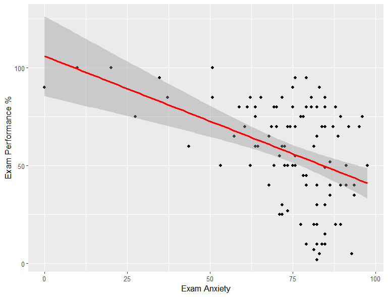
- 此时的回归线是曲线,如果想换成直线来显示回归线,
geom_smooth (method="lm")
#Simple scatter with regression line
scatter <- ggplot(examData, aes(x = Anxiety, y = Exam))
scatter +
    geom_point() +
    geom_smooth(method = "lm", colour = "Red") +
    labs(x = "Exam Anxiety", y = "Exam Performance %")
- 如果我们不想显示 95%CI, 可以 switch it off by adding "se=F"
## "se = F" means "standard error = False", can switch off the confidence interval
scatter <- ggplot(examData, aes(x = Anxiety, y = Exam))
scatter +
    geom_point() +
    geom_smooth(method = "lm", colour = "Red", se = F) +
    labs(x = "Exam Anxiety", y = "Exam Performance %")
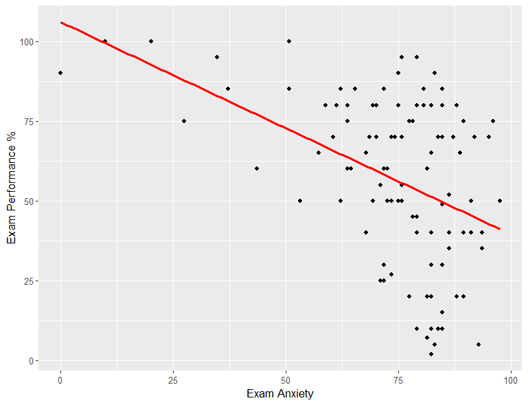
- 我们也可以改 CI shade 的填充颜色
fill = "blue", 改透明度alpha = 0.1, alpha = 1 意为不透明
#Simple scatter with regression line + colored CI
scatter <- ggplot(examData, aes(x = Anxiety, y = Exam))
scatter +
    geom_point() +
    geom_smooth(method = "lm", colour = "Red", alpha = 0.1, fill = "Red") +
    labs(x = "Exam Anxiety", y = "Exam Performance %")
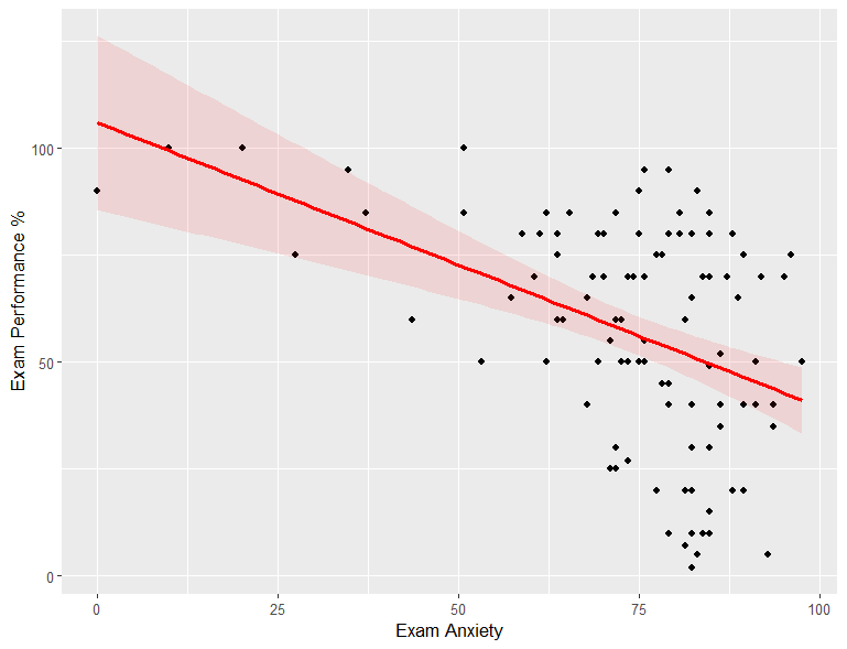
4.5.3. Grouped scatterplot
- 如果我们想看不同性别的被试的数据,可以在
ggplot(aes(color = Gender))
#Simple grouped scatter with regression line
scatter <- ggplot(examData, aes(x = Anxiety, y = Exam, color = Gender))
scatter +
    geom_point() +
    geom_smooth(method = "lm", colour = "Red") +
    labs(x = "Exam Anxiety", y = "Exam Performance %")
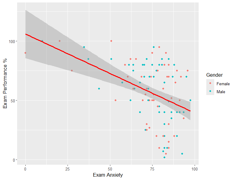
-
这时候虽然男 VS 女被试的数据有不同颜色的点表示,但是拟合线只有一条,怎么画两条呢?
-
geom_smooth(aes(color = Gender)) -
如果想用不同的颜色表示不同的拟合线,同时填充拟合线的 shade 颜色,
geom_smooth (aes(fill = Gender))
scatter <- ggplot(examData, aes(x = Anxiety, y = Exam, color = Gender))
scatter +
    geom_point() +
    geom_smooth(method = "lm", aes(fill = Gender), alpha = 0.1)
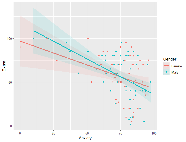
- 设置 legend 的 color 也根据 Gender 来分别呈现,在
labs(color = "Gender")【注意双引号】
scatter <- ggplot(examData, aes(x = Anxiety, y = Exam, color = Gender))
scatter +
	geom_point() +
	geom_smooth(method = "lm", aes(fill = Gender), alpha = 0.1) +
	labs(x = "Exam Anxiety", y = "Exam Performance %", color = "Gender")
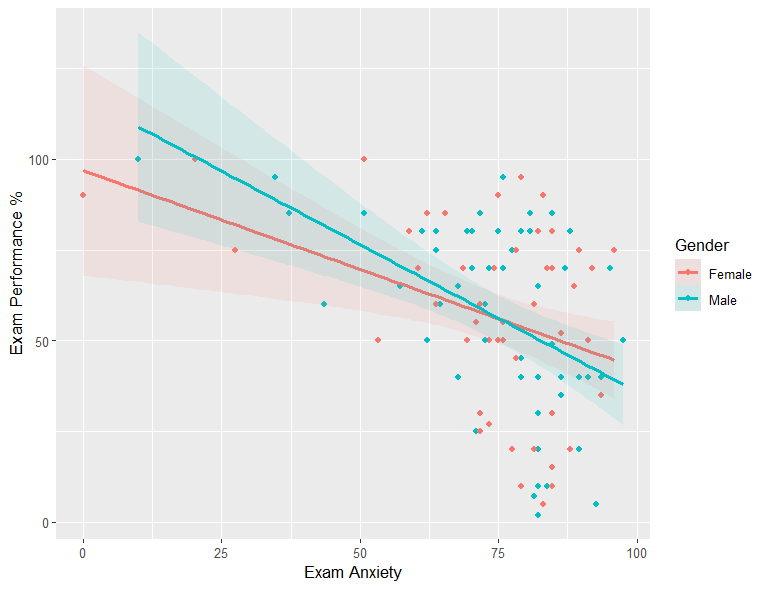
(跟上面的一样诶)
- 如果我们想自定义拟合线的填充色,可以加一层 `scale_fill_manual(values = c("#ff2bff", "#22ff22"))
scatter <- ggplot(examData, aes(x = Anxiety, y = Exam, color = Gender))
scatter +
    geom_point() +
    geom_smooth(method = "lm", aes(fill = Gender), alpha = 0.1) +
    scale_fill_manual(values = c("#22ff22", "yellow")) +
    labs(x = "Exam Anxiety", y = "Exam Performance %", color = "Gender")
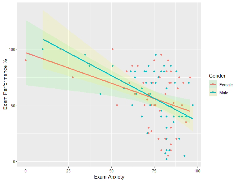
- 从图中我们能看到男性的 exam performance 更容易受到 anxiety 的负面影响(regression line 斜率负的更多)
4.6. Histograms: spot obvious problems
- 画出来的图可以清楚看到 outliers
- 其实我们 想找 outliers,有两种办法
- 一个就是画 histogram
- 另一个是求 z-scores(但这个很复杂)
- 其实我们 想找 outliers,有两种办法
#导入数据
festivalData <- read.delim("DownloadFestival.dat.txt",  header = TRUE)
festivalHistogram <- ggplot(festivalData, aes(day1)) + theme(legend.position="none")
festivalHistogram +
    geom_histogram(binwidth = 0.4) +
    labs(x = "Hygiene (Day 1 of Festival)", y = "Frequency")
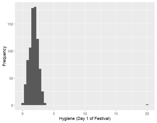
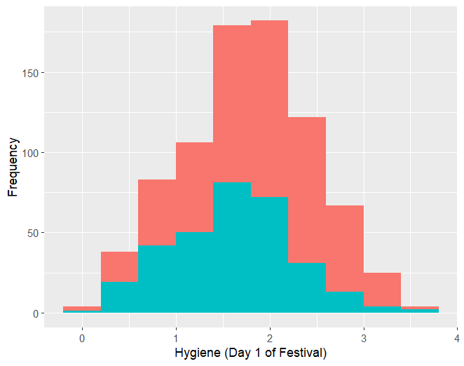
- 可以看到 Day1 的 hygiene 评分有一个值为 20 的 outlier
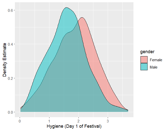
- 那我们就可以根据实际情况,考虑是否删掉这个 outlier;下面的代码是删掉 outlier 后的数据可视化,可以画 density, histogram 来展示数据的分布
festivalData2 = read.delim("DownloadFestival(No Outlier).dat.txt", header = TRUE)
festivalDensity <- ggplot(festivalData2, aes(day1))
festivalDensity +
    geom_density(aes(fill = gender), alpha = 0.5) +
    labs(x = "Hygiene (Day 1 of Festival)", y = "Density Estimate")
festivalDensity +
    geom_histogram(binwidth = 0.4, aes(fill = gender)) +
    labs(x = "Hygiene (Day 1 of Festival)", y = "Frequency") +
    theme(legend.position="none")
4.7. Boxplots (box-whisker diagrams)
ggplot(festivalData2, aes(x = gender, y = day1, fill = gender)) +
    geom_boxplot(aes(fill = gender)) +
    scale_fill_manual(values = c("violet", "green"))  +
    labs(x = "Hygiene (Day 1 of Festival)", y = "Frequency") +
    theme(legend.position="none")
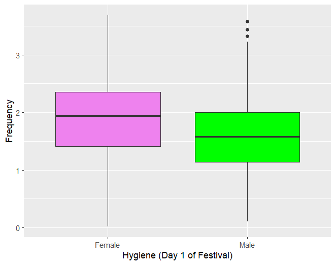
- 箱形图也能告诉我们数据是否是对称分布的,箱子是数据的 middle 50%, 箱子上部分的线是 top 25%, 箱子下部分的线是 bottom 25%;
- 如果 the range of the top and bottom 25% of scores is the same, 那么数据的 distribution is symmetrical
- 本例中,male 的数据分布比起 female 的更加 asymmetrical
4.8. Density plots
4.9. Graphing means
4.9.1. Bar charts and error bars
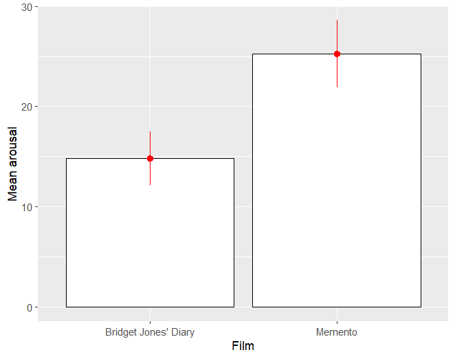
- 想探究 chick flick 电影是否对女性的吸引力更大?
- 选了两部电影,一部是代表 chick flick 的 BJ 日记,另一部是非 chick flick 的 Memento
- 招了 20 男 20 女,给 10 男 10 女看 BJ 日记,另外 10 男 10 女看 Memento,收集他们对电影的 arousal measure。
- 这个实验是个 independent design (between-subject design)
4.9.1.1. Bar charts for one independent variable
- if we want means then we have no choice but to dive in
stat., here we are usingstat_summary()to summarize the specified functions, like mean, median, mean_cl_normal
#set cran for r code running in obsidian
options(repos = c(CRAN = "https://cran.r-project.org"))

#Set the working directory (you will need to edit this to be the directory where you have stored the data files for this Chapter)
setwd("E:/R/dsur/C4exploring_data_with_graphs")

#Initiate packages
library(ggplot2)
library(reshape)
library(plyr)
# import datasets
chickFlick = read.delim("ChickFlick.dat.txt",  header = TRUE)
# if we want means then we have no choice but to dive in stat., here we are using stat_summary to summarize the specified functions
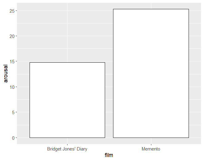
ggplot(chickFlick, aes(x = film, y = arousal)) +
    stat_summary(fun = mean, geom = "bar", fill = "white", color = "black")
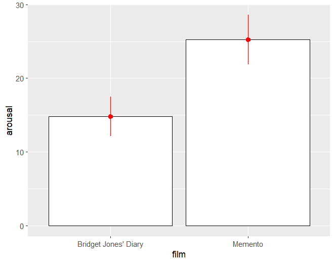
- If we want to add error bars, we can add another
stat_summary()layer, in this layer, specifyfun.data = mean_cl_normal, geom = "errorbar"或者"pointrange"
ggplot(chickFlick, aes(x = film, y = arousal)) +
    stat_summary(fun = mean, geom = "bar", fill = "white", color = "black") +
    stat_summary(fun.data = mean_cl_normal, geom = "pointrange", color = "red")
- Finally, we can add some nice labels
ggplot(chickFlick, aes(x = film, y = arousal)) +
    stat_summary(fun = mean, geom = "bar", fill = "white", color = "black") +
    stat_summary(fun.data = mean_cl_normal, geom = "pointrange", color = "red") +
    xlab("Film") +
    ylab("Mean arousal")
4.9.1.2. Bar charts for several independent variables
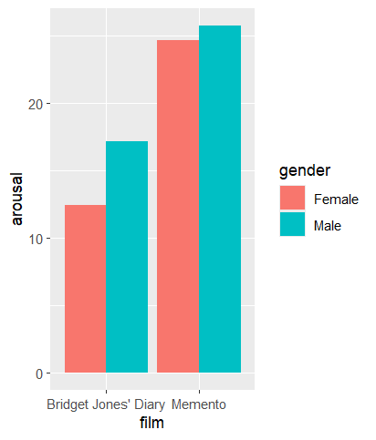
- 如果我们想看不同性别被试对两部电影的 arousal 评价,有两个办法
- 方法 1:可以在
ggplot(aes(fill = gender))- 并且,在
stat_summary(position = "dodge"), 以便较矮的 bar 不会被较高的 bar 覆盖
- 并且,在
ggplot(chickFlick, aes(x = film, y = arousal, fill = gender)) +
    stat_summary(fun = mean, geom = "bar", position = "dodge")
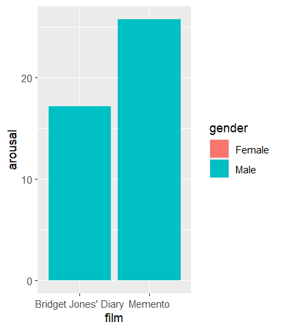
- 否则,会变成这样
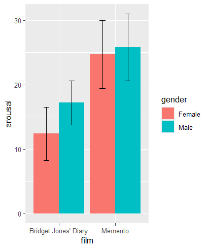
- 加上 errorbars, 这里的 position_dodge(width = 0.9) 是 errorbar 的竖线之间的宽度,width = 0.2 是 errorbar 的两端横线的宽度
ggplot(chickFlick, aes(x = film, y = arousal, fill = gender)) +
    stat_summary(fun = mean, geom = "bar", position = "dodge") +
    stat_summary(fun.data = mean_cl_normal, geom = "errorbar", position = position_dodge(width = 0.9), width = 0.2)
- 最后加上 labels
ggplot(chickFlick, aes(x = film, y = arousal, fill = gender)) +
    stat_summary(fun = mean, geom = "bar", position = "dodge") +
    stat_summary(fun.data = mean_cl_normal, geom = "errorbar", position = position_dodge(width = 0.9), width = 0.2) +
    xlab("Film") +
    ylab("Mean arousal")
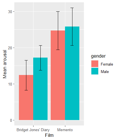
- 方法 2:用
facet_wrap(~gender), 此时ggplot(aes(fill = film))
ggplot(chickFlick, aes(x = film, y = arousal, fill = film)) +
    stat_summary(fun = mean, geom = "bar", position = "dodge") +
    stat_summary(fun.data = mean_cl_normal, geom = "errorbar", width = 0.2) +
    facet_wrap(~gender) +
    xlab("Film") +
    ylab("Mean arousal") +
    theme(legend.position = "none")
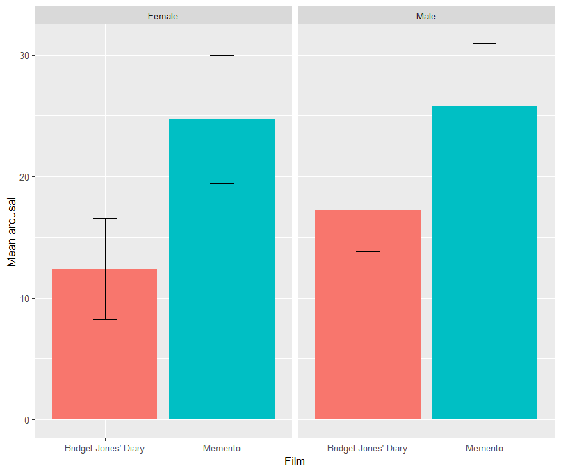
- Plot25 和 plot27 都说明了男性对 BJ 日记有更高的 arousal,而男女对 Memento 的 arousal 水平差不多;说明"chick flick"可能并不是绝对地更吸引女性观看。
4.9.2. Line graphs
4.9.2.1. Line graphs of a single independent variable
- 想探究治疗打嗝 hiccups 的 3 种方法哪种更有效
- 选了 15 名 hiccup sufferers
- 先记录没有施加治疗的 number of hiccups baseline
- 给他们施以 3 种方法(randomized order 乱序),每种方法之间隔 5mins;每种方法结束后的一分钟,记录他们的 numbers of hiccups
- 这是个 repeated-measures design
Hicccups.dat是个 wide format 的数据集- 为了让数据能够符合 ggplot 的绘图要求,我们要把 wide format 转换成 long format
#Initiate ggplot2
library(ggplot2)
library(reshape)
library(plyr)

#Set wd
setwd("E:/R/dsur/C4exploring_data_with_graphs")

#Import dataset
hiccupsData <- read.delim("Hiccups.dat.txt",  header = TRUE)
stack()将 wide format 转换成 long format
# transfer the wide format to long format so that ggplot2 can use
hiccups<-stack(hiccupsData)
# rename the column names
names(hiccups)<-c("Hiccups","Intervention")
- 把
"Intervention"列变成 factor,这样便于分组和查找- To avoid duplicated troubles, use
unique()
- To avoid duplicated troubles, use
# transfer "Intervention" as a factor, meanwhile rename it as "Intervention_Factor"
## to avoid duplicated troubles, use unique()
hiccups$Intervention_Factor<-factor(hiccups$Intervention, levels = unique(hiccups$Intervention))
- 现在,可以画图了
# we can plot the means of each intervention
ggplot(hiccups, aes(x = Intervention_Factor, y = Hiccups)) +
    stat_summary(fun = mean, geom = "point")
# we want to add a line to connect the means point to show the difference
ggplot(hiccups, aes(x = Intervention_Factor, y = Hiccups)) +
    stat_summary(fun = mean, geom = "point") +
    stat_summary(fun = mean, geom = "line", aes(group = 1)) #aes(group = 1) means to connect 4 means points as a line, but it doesnt matter about the number, just put a constant in 你可以在 `aes()` 内添加 `group = 1`,这会让 `geom_line()` 将所有数据点视为一个组,从而绘制出正确的连线
# we want to modify the line color and linetype
ggplot(hiccups, aes(x = Intervention_Factor, y = Hiccups)) +
    stat_summary(fun = mean, geom = "point") +
    stat_summary(fun = mean, geom = "line", aes(group = 1), color = "blue", linetype = "dashed")
# we want to add errorbars
ggplot(hiccups, aes(x = Intervention_Factor, y = Hiccups)) +
    stat_summary(fun = mean, geom = "point") +
    stat_summary(fun = mean, geom = "line", aes(group = 1), color = "blue", linetype = "dashed") +
    stat_summary(fun.data = mean_cl_normal, geom = "errorbar", color = "green", width = 0.2)
# we want to add xlab and y lab
ggplot(hiccups, aes(x = Intervention_Factor, y = Hiccups)) +
    stat_summary(fun = mean, geom = "point") +
    stat_summary(fun = mean, geom = "line", aes(group = 1), color = "blue", linetype = "dashed") +
    stat_summary(fun.data = mean_cl_normal, geom = "errorbar", color = "green", width = 0.2) +
    xlab("Intervention") +
    ylab("Mean number of hiccups")
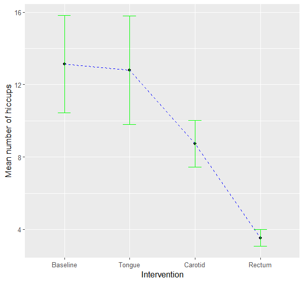
-
so the graph can tell us: the effectiveness of Rectum is the best, so if you have hiccups, find something digital and amuse yourself for a few minutes
-
如果我们想改变 4 个列的呈现位置,可以在
factor(levels()[c()])用一个向量c()指定顺序- The original order in hiccups is Baseline-1, Tongue-2, Carotid-3, Rectum-4
- But we can define the order as c (1, 4, 2, 3) 所以原来在 4 位置的 Rectum 会被移到第二列进行图形展示,Tongue 被移到第三列进行展示,Carotid 被移到第四列
hiccups$Intervention_Factor<-factor(hiccups$Intervention, levels(hiccups$Intervention)[c(1, 4, 2, 3)])
- 这样之后,画图还是用上面的同样代码
# we can see the order of representation has been changed
ggplot(hiccups, aes(x = Intervention_Factor, y = Hiccups)) +
    stat_summary(fun = mean, geom = "point") +
    stat_summary(fun = mean, geom = "line", aes(group = 1), color = "blue", linetype = "dashed") +
    stat_summary(fun.data = mean_cl_normal, geom = "errorbar", color = "green", width = 0.2) +
    xlab("Intervention") +
    ylab("Mean number of hiccups")
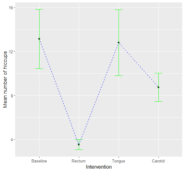
- 这时候,数据的列呈现顺序就变了
4.9.2.2. Line graphs for several independent variables
- 探究手机发消息是否对学生的语法水平有影响,
- 召集了 2 组学生,每组 25 人
- 其中一组允许他们在 6 个月内使用手机发消息,另一组不允许发消息
- 在干预之前和之后测他们的语法水平
- 这是个 mixed design
- Between-subject factor: 是否允许发消息
- Within-subject factor: 干预之前和之后,两组人都要接受语法水平测试
- 召集了 2 组学生,每组 25 人
- 所以,我们会比较两组人的数据(干预前& 干预后),那么要把两个 factors 呈现在一个图里
- 先设置工作路径,导入数据
#Initiate ggplot2
library(ggplot2)
library(reshape)
library(plyr)

#Set wd
setwd("E:/R/dsur/C4exploring_data_with_graphs")

#Import dataset
textData <- read.delim("TextMessages.dat.txt",  header = TRUE)
head(textData)
- 但是,this is a wide format data, we need to transfer it into long format so that ggplot2 can use
- 给每一行附上一个 id,方便后续数据追踪
textData$id <- row(textData[1])
- 把 Group 转换成 factor
factor()
textData$Group_factor <- factor(textData$Group, levels = unique(textData$Group))
- Reshape the data from wide to long--method1
textMessages <- reshape(textData, # 要转换的原始数据框
                        idvar = c ("id", "Group_factor"),  # 用于唯一标识每个参与者的列(id和Group)
                        varying = c("Baseline", "Six_months"), # 需要转换的宽格式列,这些列将合并为一列
                        v.names = "Grammar_Score", # 新生成的列名,用于存储合并后的“语法分数”
                        timevar = "Time", # 新生成的时间变量列名,用于区分数据时间点
                        times = c(0:1), # 指定时间点,0表示Baseline,1表示Six_months;这里的数字不重要,若写成 times = c(1:2)那生成的数据框就是用1表示Baseline, 2表示Six_months
                        direction = "long") # 指定转换方向为长格式
### transfer Time as a factor
textMessages$Time_factor <- factor(textMessages$Time, labels = c("Baseline", "After"))
- 我也可以在 reshape ()的时候写成
times = c ("Baseline", "After"), 这样 factor ()的时候可以不用写labels = c ("Baseline", "After")
# textMessages1 <- reshape(textData,
#                         idvar = c ("id", "Group_factor"),
#                         varying = c("Baseline", "Six_months"),
#                         v.names = "Grammar_Score",
#                         timevar = "Time",
#                         times = c("Baseline", "After"),
#                         direction = "long")
# textMessages1$Time_factor <- factor(textMessages1$Time, levels = unique(textMessages1$Time))
- Reshape the data from wide to long--method2
# textMessages <- melt(textData, id = c("id", "Group"), measured = c("Baseline", "Six_months"))
# names(textMessages) <- c("id", "Group", "Time", "Grammar_Score")
# textMessages$Time <- factor(textMessages$Time, labels = c("Baseline", "After"))
- 现在,我们可以画图了
#plot the line graphs
ggplot(textMessages, aes(x = Time_factor, y = Grammar_Score, color = Group_factor)) +
    stat_summary(fun = mean, geom = "point", shape = 9, size = 2) +
    stat_summary(fun = mean, geom = "line", aes(group = Group_factor, linetype = Group_factor)) + # add line to connect points, 不同的组用不同的连接线样式
    stat_summary(fun.data = mean_cl_boot, geom = "errorbar", width = 0.5, size = 1) + # add errorbars using fun.data = mean_cl_boot
    xlab("Time") +
    ylab("Mean Grammar Score")
- 在 ggplot2 包中的
stat_summary()函数中,mean_cl_normal和mean_cl_boot是用于计算平均值及其置信区间(CI)的统计方法。mean_cl_normal:计算正态分布假设下的置信区间(Normal CI)。此方法假设数据分布为正态分布,使用标准误差来计算置信区间,适用于数据量大、接近正态分布的情况。mean_cl_boot:计算自助法Bootstrapped置信区间(Bootstrapped CI)。自助法通过在样本中反复抽样来估计置信区间,适用于数据不完全正态或数据量较少的情况。它无需正态分布假设,因此在数据偏态或样本较小的情况下可能更可靠。
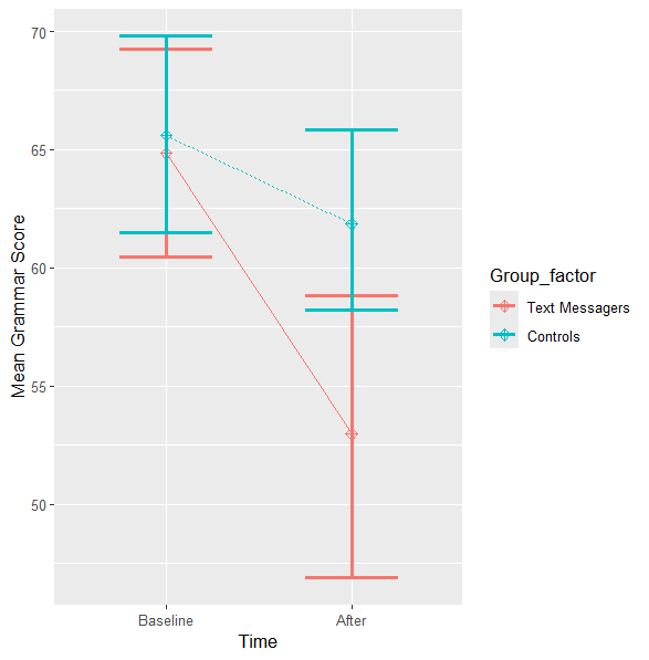
- 从图中我们可以得到结论:用手机发消息的那组人在 6 个月后,语法水平下降得很多,所以,用手机发消息对写作不好呀
4.10. Themes and options
- 两个默认的 themes
theme_gray()和theme_bw()
- 但我们也可以自定义主题来设置背景 grid 的线条颜色、linetype,size
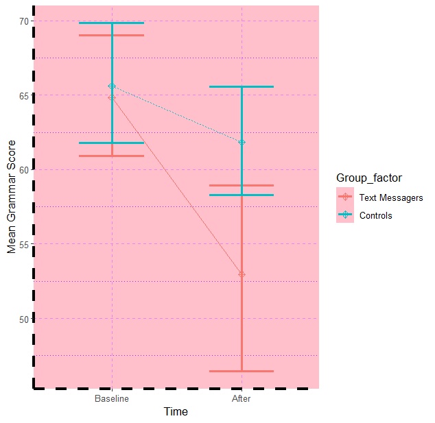
- follow up 上面的图,我们可以加上
theme()layers
ggplot(textMessages, aes(x = Time_factor, y = Grammar_Score, color = Group_factor)) +
    stat_summary(fun = mean, geom = "point", shape = 9, size = 2) +
    stat_summary(fun = mean, geom = "line", aes(group = Group_factor, linetype = Group_factor)) + # add line to connect points, 不同的组用不同的连接线样式
    stat_summary(fun.data = mean_cl_boot, geom = "errorbar", width = 0.5, size = 1) + # add errorbars using fun.data = mean_cl_boot
    xlab("Time") +
    ylab("Mean Grammar Score") +
    theme(panel.grid.major = element_line(color = "violet", linetype = 2)) + #背景的大格子线条颜色和样式
    theme(panel.grid.minor = element_line(color = "purple", linetype = 3)) + #背景的小格子线条颜色和样式
    theme(panel.background = element_rect(fill = "pink")) + #背景填充颜色
    theme(axis.line = element_line(color = "black", linetype = 2, size = 1.5)) #坐标轴线条的颜色和样式
Smart Alex's tasks
Task 1
-
Using the data from chapter 3, plot and interpret the following graphs
-
- An error bar chart showing the mean number of friends for students and lecturers
-
- An error bar chart showing the mean alcohol consumption for students and lecturers
-
- An error line chart showing the mean income for students and lecturers
-
- An error line chart showing the mean neuroticism for students and lecturers
-
- A scatterplot with regression lines of alcohol consumption and neuroticism grouped by lecturer/student
-
-
回答
-
导入数据
lecturerData = read.delim("Lecturer Data.dat.txt", header = TRUE)
- 将 job 转换成 factor
lecturerData$job_factor <- factor(lecturerData$job, labels = c("lecturer", "student"))
friends_comparison <-
    ggplot(lecturerData, aes(x = job_factor, y = friends, color = job_factor)) +
        stat_summary(fun = mean, geom = "bar") +
        stat_summary(fun.data = mean_cl_boot, geom = "errorbar", width = 0.5) +
        xlab("Job")+
        ylab("Number of Friends") +
        theme(legend.position = "none")
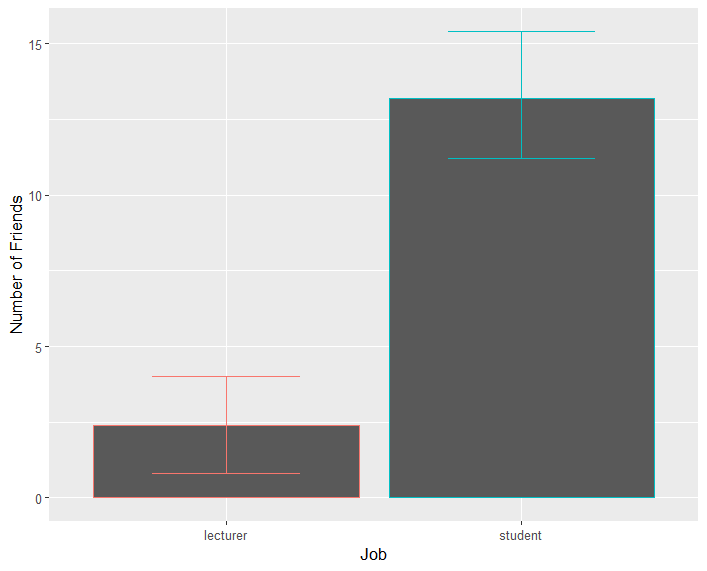
-
Lecturer 人群的朋友少,好可怜🙁
-
alcohol_comparison <-
    ggplot(lecturerData, aes(x = job_factor, y = alcohol, color = job_factor)) +
        stat_summary(fun = mean, geom = "bar") +
        stat_summary(fun.data = mean_cl_boot, geom = "errorbar", width = 0.5) +
        xlab("Job")+
        ylab("Alcohol Consumption") +
        theme(legend.position = "none")
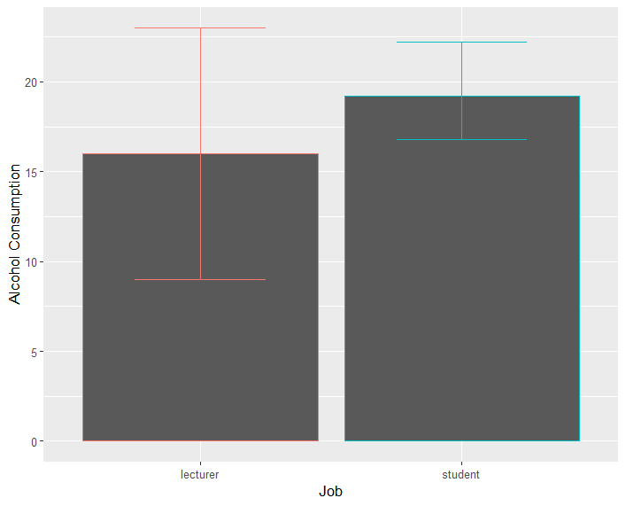
-
学生的平均喝酒量比 lecturer 多
-
income_comparison <-
    ggplot(lecturerData, aes(x = job_factor, y = income, color = job_factor)) +
        stat_summary(fun = mean, geom = "point", size = 2) +
        stat_summary(fun = mean, geom = "line", aes(group = 2), color = "blue", linetype = 2) +
        stat_summary(fun.data = mean_cl_boot, geom = "errorbar", width = 0.5) +
        xlab("Job")+
        ylab("Income") +
        theme(legend.position = "none")
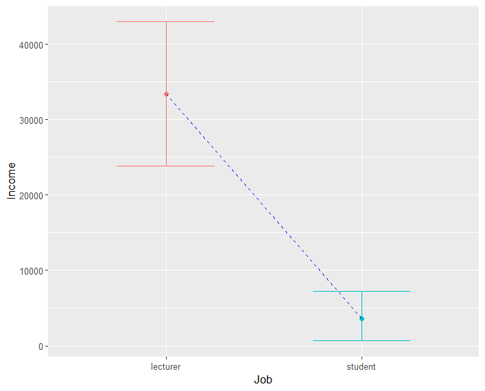
-
lecturer 的收入比学生高很多,而且 lecturer 的收入变异量比学生人群的大
-
neurotic_comparison <-
    ggplot(lecturerData, aes(x = job_factor, y = neurotic, color = job_factor)) +
        stat_summary(fun = mean, geom = "point", size = 2) +
        stat_summary(fun = mean, geom = "line", aes(group = 2), color = "blue", linetype = 2) +
        stat_summary(fun.data = mean_cl_boot, geom = "errorbar", width = 0.5) +
        xlab("Job")+
        ylab("Neurotic Measure") +
        theme(legend.position = "none")
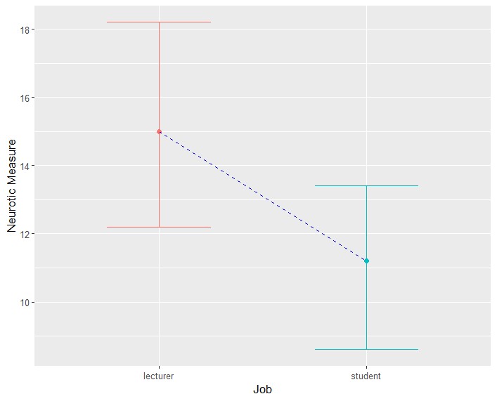
-
lecturer 人群的神经质水平比学生人群高(读书读傻了😄
-
scatter_alcohol_neurotic <-
    ggplot(lecturerData, aes(x = neurotic, y = alcohol, group = job_factor, color = job_factor)) +
        geom_point() +
        geom_smooth(method = "lm", aes(fill = job_factor), alpha = 0.1) +
        scale_fill_manual(values = c("#ffb385", "#000055")) + #填充CI的颜色
        scale_color_manual(values = c("#ffb385", "#000055")) +  #填充拟合线的颜色
        xlab("Neurotic Measure") +
        ylab("Alcohol Consumption")
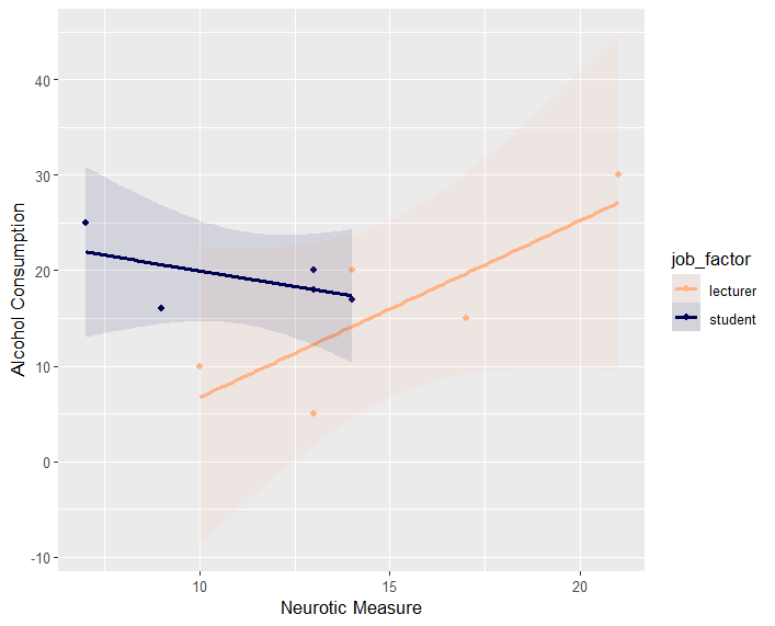
- 从图中,可以得知,lecturer 的神经质水平与喝的酒是正相关关系,喝酒越多,越神经质;越神经质,喝酒越多;
而 students 的神经质与喝酒量呈负相关
Task 2
-
Using the Infidelity data from chapter 3, plot a clustered error bar chart of the mean number of bullets used against self and partner for males and females
-
回答
-
导入数据
infidelityData <- read.csv("Infidelity.csv", header = TRUE)
- Transfer wide format to long format
infidelityData$id <- row(infidelityData[1])
## make Gender as a factor
infidelityData$Gender_factor <- factor(infidelityData$Gender, levels = unique(infidelityData$Gender))
infidelity_long <- reshape(infidelityData,
                           idvar = c("id", "Gender_factor"),
                           varying = c("Partner", "Self"),
                           v.names = "Bullet_number",
                           timevar = "Target",
                           times = c(0:1), #"Partner--0" "Self--1"
                           direction = "long")
- Make Target as a factor
infidelity_long$Target_factor <- factor(infidelity_long$Target, labels = c("Partner", "Self"))
- Make the scatter plot
ggplot(infidelity_long, aes(x = Target_factor, y = Bullet_number, group = Gender_factor, color = Gender_factor)) +
    stat_summary(fun = mean, geom = "bar", position = "dodge", aes(fill = Gender_factor)) +
    stat_summary(fun.data = mean_cl_boot, geom = "errorbar", position = position_dodge(width = 0.9), width = 0.2) +
    scale_fill_manual(values = c("#ffb385", "#000055")) + #填充色
    #scale_color_manual(values = c("red", "green")) +  #轮廓线颜色
    xlab("Targets") +
    ylab("Number of Bullets")
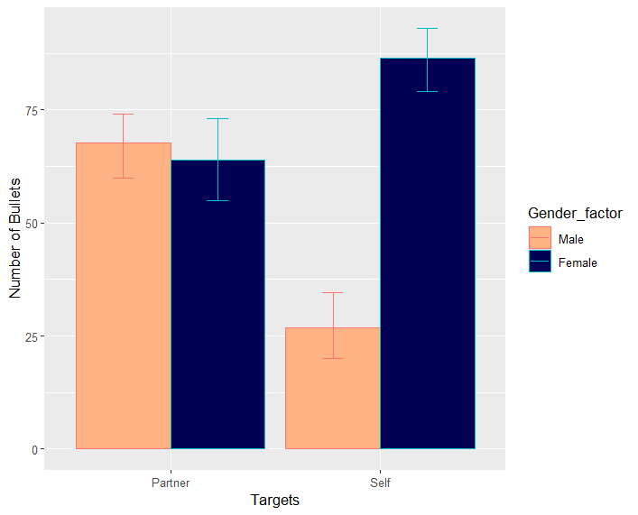
- 从图中可知,男性得知配偶出轨后,射杀配偶的可能性大于自杀,
而女性得知配偶出轨后,自杀的可能性大于射杀配偶;(何苦呢女人)
在射杀配偶的情况下,男性射出去的子弹与女性射出去的子弹数量差别不大,
可是在自杀的情况下,女性射出去的子弹数量远远大于男性 (女人对自己真狠啊)
C5. Exploring assumptions
5.1. What will this chapter tell me?
- 丑小鸭的故事
- Data 就像丑小鸭,一开始拿到手时,they are big, grey and ugly. We swear at them, curse them, peck them and hope that they'll fly away and be killed by the swans.
- 但是, we can try to force our data into becoming beautiful swans
- 本章就是:assess how much of an ugly duckling of a data set you have, and discover how to turn it into a swan.
5.3. Assumptions of parametric data
- 大部分的 statistical procedures in this book are parametric tests (based on the normal distribution))
- Parametric test:
- 需要的 data 是属于统计学家已经定义好的 distributions; 如 normal distribution
- Certain assumptions must be true -> data to be parametric (如果你的 data are not parametric, 但你用了 parametric tests, 那结果很可能 inaccurate)
- Parametric test:
- 基于正态分布的 parametric tests 有 4 basic assumptions that must be met for the test to be accurate
- Normally distributed data
- The rationale behind hypothesis testing relies on having something that is normally distributed
- In some cases it is the sampling distribution
- In others the errors in the model (regression models; GLM)
- If this assumption is not met → the logic behind hypothesis testing is flawed
- The rationale behind hypothesis testing relies on having something that is normally distributed
- Homogeneity of variance
- The variances should be the same throughout the data
- 若实验设计找了多组被试,则方差齐性检验指的就是:each of these samples comes from populations with the same variance (被试来自的 populations 变异都相同)
- 若是相关性设计,则方差齐性检验指的是:the variance of one variable should be stable at all levels of the other variable
- Interval data
- data should be measured at least at the interval level
- Independence
- Data from different participants are independent: the behavior of one participant does not influence the behavior of another
- In repeated-measures designs: behavior between different participants should be independent, 而同一个被试的不同实验条件下的 scores 是 non-independent
同一个被试接受所有条件的测试,改被试的行为之间不是独立的,但不同被试的行为是独立的 - In regression: the errors in the regression model should be uncorrelated
这里的 errors 就是 #2.4.2. Assessing the fit of the mean sums of squares 平方和, variance 方差, SD 标准差 中的 deviations
- Normally distributed data
- 本章主要是讲 normality & homogeneity of variance
5.4. Packages used in this chapter
install.packages("car")
install.packages("ggplot2")
install.packages("pastecs")
install.packages("psych")

library(car)
library(ggplot2)
library(pastecs)
library(psych)
5.5. The assumption of normality
- 我们不能直接看到 population 的 distribution,但根据 central limit theorem 中心极限定理
- If the sample data is normal, then the sampling distribution will be so
- 所以,通常都要先看自己收的 sample data 是否 normal
- 而且,中心极限定理告诉我们,在 big samples 中,distribution tends to be normal
- 在用 regression or GLM 时,the assumption of normality 尤为重要
5.5.1. Checking normality visually
- Read
"DownloadFestival.dat.txt"数据集
setwd("E:/R/dsur/C5exploring_assumptions")
imageDirectory <- "E:/R/dsur/C5exploring_assumptions/images"

#Read in the download data:

dlf <- read.delim("DownloadFestival.dat.txt", header=TRUE)
names(dlf)
View(dlf)
#day1列有一个20 .02的异常值 outlier,我们要把它给改成 NA
#Remove the outlier from the day1 hygiene score
dlf$day1 <- ifelse(dlf$day1 > 20, NA, dlf$day1)
- 画直方图,看数据的分布
- After_stat (density) 直接引用统计变换后的变量:密度;这里的 density 可以换成 count (计数)或 prop (比例)
- density 是相对于数据的分布概率密度(相对频率)进行标准化,
而不是直接显示数据的计数 count, 只有这样才能与正态模型进行比对,才能加上正确的 normal curve
Below 的代码显示的是默认 count 的直方图,但想加 normal curve,却不是我们想要的,这里会紧贴 x 轴,因为 normal curve 的 y 值在 0-1 之间
hist.day11 <- ggplot(dlf, aes(day1)) +
    geom_histogram(color = "black", fill = "white") +
    theme(legend.position = "none") +
    stat_function(fun = dnorm, args = list(mean = mean(dlf$day1, na.rm = TRUE), sd = sd(dlf$day1, na.rm = TRUE)), color = "blue", linewidth = 0.5) +
    labs(x = "Hygiene score on day 1", y = "Count")
hist.day11
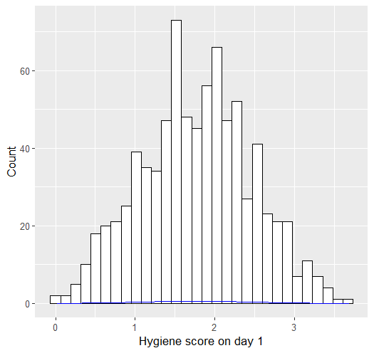
- 画 day1 数据的 density 直方图
hist.day1 <- ggplot(dlf, aes(day1)) +
    geom_histogram(aes(y = after_stat(density)), color = "black", fill = "white") +
    theme(legend.position = "none") +
    labs(x = "Hygiene score on day 1", y = "Density")
hist.day1
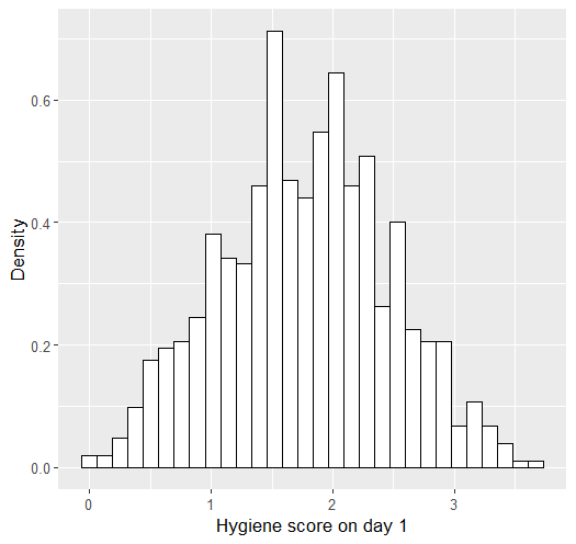
- 同理,画 day2, day3 的
#Histogram for day 2:
hist.day2 <- ggplot(dlf, aes(day2)) +
    geom_histogram(aes(y = after_stat(density)), color = "black", fill = "white") +
    theme(legend.position = "none") +
    labs(x = "Hygiene score on day 2", y = "Density")
hist.day2

#Histogram for day 3:
hist.day3 <- ggplot(dlf, aes(day3)) +
    geom_histogram(aes(y = after_stat(density)), color = "black", fill = "white") +
    theme(legend.position = "none") +
    labs(x = "Hygiene score on day 2", y = "Density")
hist.day3
- Add the curves to the Histograms: add a layer
stat_function()
#Histogram for day1 with a norm curve:
hist.day1 <- ggplot(dlf, aes(day1)) +
    geom_histogram(aes(y = after_stat(density)), color = "black", fill = "white") +
    stat_function(fun = dnorm, args = list(mean = mean(dlf$day1, na.rm = TRUE), sd = sd(dlf$day1, na.rm = TRUE)), color = "blue", linewidth = 0.5) +
    theme(legend.position = "none") +
    labs(x = "Hygiene score on day 1", y = "Density")
hist.day1
ggsave(file = paste(imageDirectory,"05_dlf_day1_hist.png",sep="/"))
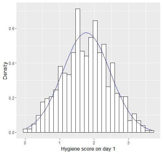
#Histogram for day2 with a norm curve:
hist.day2 <- ggplot(dlf, aes(day2)) +
    geom_histogram(aes(y = after_stat(density)), color = "black", fill = "white") +
    stat_function(fun = dnorm, args = list(mean = mean(dlf$day2, na.rm = TRUE), sd = sd(dlf$day2, na.rm = TRUE)), color = "blue", linewidth = 0.5) +
    theme(legend.position = "none") +
    labs(x = "Hygiene score on day 2", y = "Density")
hist.day2
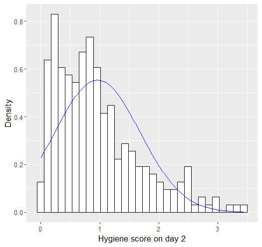
#Histogram for day3 with a norm curve:
hist.day3 <- ggplot(dlf, aes(day3)) +
    geom_histogram(aes(y = after_stat(density)), color = "black", fill = "white") +
    stat_function(fun = dnorm, args = list(mean = mean(dlf$day3, na.rm = TRUE), sd = sd(dlf$day3, na.rm = TRUE)), color = "blue", linewidth = 0.5) +
    theme(legend.position = "none") +
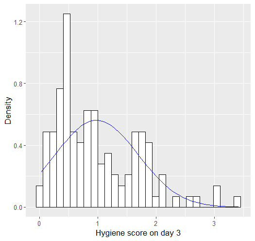
    labs(x = "Hygiene score on day 3", y = "Density")
hist.day3
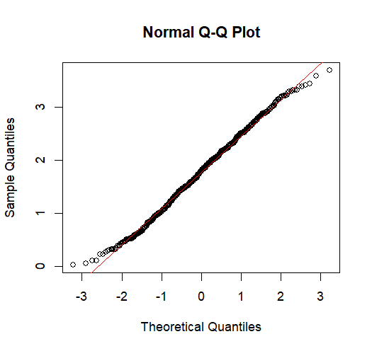
- 除了直方图,我们也可以画 q-q plot 来看是否正态分布
#Q-Q plot for day 1:
qqnorm(dlf$day1)
qqline(dlf$day1, col = "red")
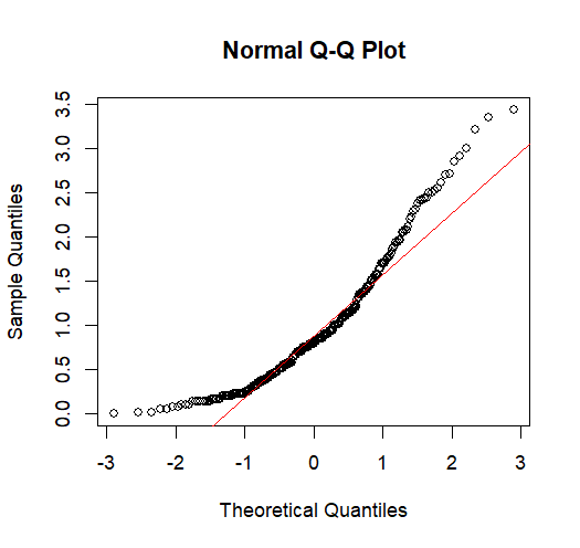
#Q-Q plot for day 2:
qqnorm(dlf$day2)
qqline(dlf$day2, col = "red")
#Q-Q plot of the hygiene scores on day 3:
qqnorm(dlf$day3)
qqline(dlf$day3, col = "red")
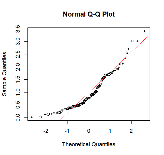
- 从以上的直方图和 q-q 图我们都可以看出, day1 的数据,比起 day2 和 day3 的,更正态分布
- Day2 & day3 的数据看起来是 positively skewed
- 这种 skewed distribution 会在我们执行 parametric tests 的时候带来麻烦,所以我们要知道 skewness & kurtosis 具体是多少数值 → #5.5.2. Quantify normality with numbers
5.5.2. Quantify normality with numbers
- Use
describe()in"psych"package - Or
stat.desc()in"pastecs"package e的含义9.612e-02即把小数点往左移 2 位 = 0.096129.612e-01即把小数点往左移 1 位 = 0.96129.612e+02即把小数点往右移 2 位 = 961.2
- 要看 skewness & kurtosis values
- Normal distribution 的 skewness = 0, kurtosis = 0
- 当然,也可以把 skewness & kurtosis 转换为 z-score, 这样就可以与任何偶然获得的数据进行比较
- Z-score 之后的数据 【这时是与标准的 normal distribution model 进行比较,看我们的 data 是否 normal】
- 若绝对值>1.96, 则在 p<0.05 的情况下 sign.
- 若绝对值>2.58, 则在 p<0.01 的情况下 sign.
- 若绝对值>3.29, 则在 p<0.001 的情况下 sign.
- 样本量较小的情况,用 p=0.05 就够了;但是当 sample size≥200 时,用 p=0.01 甚至 p=0.001 都不为过
- 【注意:当 sample size ≥ 200 时,先画图出来看 shape of the distribution 很重要,而不是一上来就直接计算 sign.】
stat.desc()除了输出 skewness, kurtosis 的值之外,还会输出skew. 2SE和kurt.2SE, 这两个是 skew & kurtosis 的 value divided by 2 SEs- 上面说了 z-score 后的 skew & kurtosis 若>1.96(或者说>2),就是 sign. 数据 non-normal
那么直接在 z-score 上除以 2,即 skew. 2SE, 那么就看这个值是否>1 就可以判断是否 sign. 了- 若
skew.2SE或kurt.2SE的绝对值-
1, (p<0.05), sign., 数据 non-normal
-
1.29, (p<0.01), sign., 数据 non-normal
-
1.65, (p<0.001), sign., 数据 non-normal
-
- 若
- 此外,
stat.desc()还可以告诉我们 shapiro-wilk test (检验是否正态分布) 的结果,normtest.Wnormtest.p,详细见 #
- 上面说了 z-score 后的 skew & kurtosis 若>1.96(或者说>2),就是 sign. 数据 non-normal
- 把输出结果的数字小数点改少|多,用
round()round(object we want to round, digits = x)
### 5.5.2. Quantifying normality with numbers
library(psych)		#load the psych library, if you haven't already, for the describe() function.

#Using the describe() function for a single variable.
describe(dlf$day1)

#Two alternative ways to describe multiple variables.
describe(cbind(dlf$day1, dlf$day2, dlf$day3)) # cbind()把需要的数据列按列拼接,如果直接写describe(dlf)也可以得到想要的结果,但是会把gender和ticknumb列也描述出来
describe(dlf[,c("day1", "day2", "day3")])

#Using the stat.desc() function for a single variable
library(pastecs) #stat.desc() function is from the pastecs package
stat.desc(dlf$day1, basic = FALSE, norm = TRUE)

#Two alternative ways to describe multiple variables.
stat.desc(cbind(dlf$day1, dlf$day2, dlf$day3), basic = FALSE, norm = TRUE)
stat.desc(dlf[, c("day1", "day2", "day3")], basic = FALSE, norm = TRUE)

round(stat.desc(dlf[, c("day1", "day2", "day3")], basic = FALSE, norm = TRUE), digits = 3)
5.5.3. Exploring groups of data
by()subset()
5.5.3.1. Running the analysis for all data
- 之前也说过,
describe()stat.desc()可以告诉我们 instant distribution of our data, 能看skew.2SE或kurt.2SE的值,从而告诉我们哪些数据是 skewed | kurtosis
#Read in R exam data.
rexam <- read.delim("rexam.dat.txt", header=TRUE)

#Set the variable uni to be a factor: 0 means Duncetown Uni, 1 means Sussex Uni
rexam$uni<-factor(rexam$uni, levels = c(0:1), labels = c("Duncetown University", "Sussex University"))

#Self-test task
#descriptive stats of the rexam dataset
describe(rexam[, c("exam", "computer", "numeracy", "lectures")])
stat.desc(cbind(rexam$exam, rexam$computer, rexam$numeracy, rexam$lectures), basic = FALSE, norm = TRUE)
round(stat.desc(rexam[, c("exam", "computer", "numeracy", "lectures")], basic = FALSE, norm = TRUE), digits = 3)
round(stat.desc(rexam[, c("exam", "computer", "numeracy", "lectures")], basic = FALSE, norm = TRUE), digits = 3)
exam computer numeracy lectures
median 60.000 51.500 4.000 62.000
mean 58.100 50.710 4.850 59.765
SE.mean 2.132 0.826 0.271 2.168
CI.mean.0.95 4.229 1.639 0.537 4.303
var 454.354 68.228 7.321 470.230
std.dev 21.316 8.260 2.706 21.685
coef.var 0.367 0.163 0.558 0.363
skewness -0.104 -0.169 0.933 -0.410
skew.2SE -0.215 -0.350 1.932 -0.849
kurtosis -1.148 0.221 0.763 -0.285
kurt.2SE -1.200 0.231 0.798 -0.298
normtest.W 0.961 0.987 0.924 0.977
normtest.p 0.005 0.441 0.000 0.077
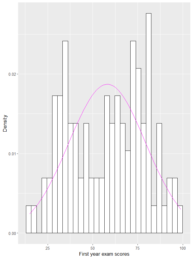
然后,我们画直方图
#draw histograms
hist.exam <- ggplot(rexam, aes(exam)) +
    geom_histogram(aes(y = after_stat(density)), color = "black", fill = "white") +
    stat_function(fun = dnorm, args = list(mean = mean(rexam$exam, na.rm = TRUE), sd = sd(rexam$exam, na.rm = TRUE)), color = "#fc00fc", linewidth = 0.5) +
    theme(legend.position = "none") +
    labs(x = "First year exam scores", y = "Density")
hist.exam
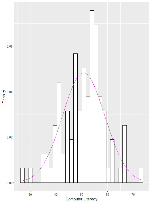
hist.computer <- ggplot(rexam, aes(computer)) +
    geom_histogram(aes(y = after_stat(density)), color = "black", fill = "white") +
    stat_function(fun = dnorm, args = list(mean = mean(rexam$computer, na.rm = TRUE), sd = sd(rexam$computer, na.rm = TRUE)), color = "#fc00fc", linewidth = 0.5) +
    theme(legend.position = "none") +
    labs(x = "Computer Literacy", y = "Density")
hist.computer
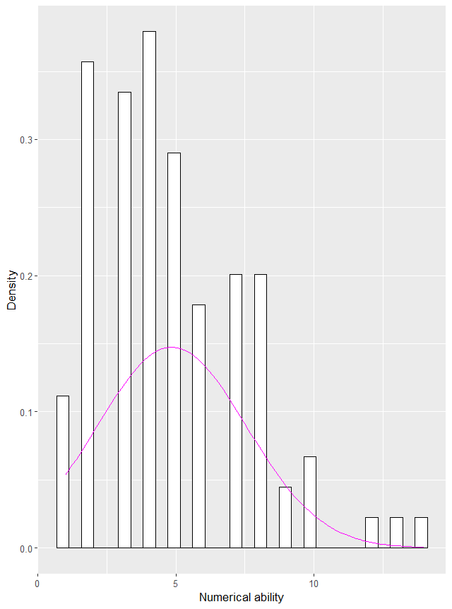
hist.numeracy <- ggplot(rexam, aes(numeracy)) +
    geom_histogram(aes(y = after_stat(density)), color = "black", fill = "white") +
    stat_function(fun = dnorm, args = list(mean = mean(rexam$numeracy, na.rm = TRUE), sd = sd(rexam$numeracy, na.rm = TRUE)), color = "#fc00fc", linewidth = 0.5) +
    theme(legend.position = "none") +
    labs(x = "Numerical ability", y = "Density")
hist.numeracy
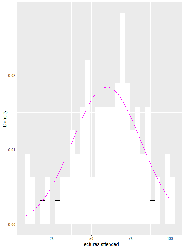
hist.lectures <- ggplot(rexam, aes(lectures)) +
    geom_histogram(aes(y = after_stat(density)), color = "black", fill = "white") +
    stat_function(fun = dnorm, args = list(mean = mean(rexam$lectures, na.rm = TRUE), sd = sd(rexam$lectures, na.rm = TRUE)), color = "#fc00fc", linewidth = 0.5) +
    theme(legend.position = "none") +
    labs(x = "Lectures attended", y = "Density")
hist.lectures
5.5.3.2. Running the analysis for different groups
- Use
by()to get descriptives for one variable, split by uni by(data = rexam$exam, INDICES = rexam$uni, FUN = describe)也可以省略默认位置的提示词写成by(rexam$exam, rexam$uni, describe)
- 同理,如果 function 是用
stat.desc(),就在相应位置修改即可 - 下面这个
basic = False意思是不想要输出 basic statistics,norm = TRUE意思是要输出 normality statistics - `by(rexam
uni, stat.desc, basic = FALSE, norm = TRUE)
#若想得到不同组别的多个变量的descriptives,可以用cbind()来指定多个变量
by(cbind(data=rexam$exam, data=rexam$numeracy), rexam$uni, describe)
by(rexam[, c("exam", "numeracy")], rexam$uni, stat.desc, basic = FALSE, norm = TRUE)
#可以看到Sussex Uni的学生的exam平均成绩比Dunceton Uni的高36%,numeracy的分数也比较高
#Use describe for four variables in the rexam dataframe.
describe(cbind(rexam$exam, rexam$computer, rexam$lectures, rexam$numeracy))
#Use by() to get descriptives for four variables, split by uni
by(data = cbind(rexam$exam, rexam$computer, rexam$lectures, rexam$numeracy), rexam$uni, describe)
by(rexam[, c("exam", "computer", "lectures", "numeracy")], rexam$uni, stat.desc, basic = FALSE, norm = TRUE)
## round the results with 3 digits
by(
    data = rexam[, c("exam", "computer", "lectures", "numeracy")],
    INDICES = rexam$uni,
    FUN = function(subset) {
        round(
            stat.desc(subset, basic = FALSE, norm = TRUE),
            digits = 3
        )
    }
)
#Self test:
#Use by() to get descriptives for computer literacy and percentage of lectures attended, split by uni
by(cbind(data=rexam$computer, data=rexam$lectures), rexam$uni, describe)
by(rexam[, c("computer", "lectures")], rexam$uni, stat.desc, basic = FALSE, norm = TRUE)
- 分组别画 histograms 时,用
subset()把需要的数据先摘出来,然后再用ggplot()画图
#using subset to plot histograms for different groups:
dunceData<-subset(rexam, rexam$uni=="Duncetown University")
sussexData<-subset(rexam, rexam$uni=="Sussex University")

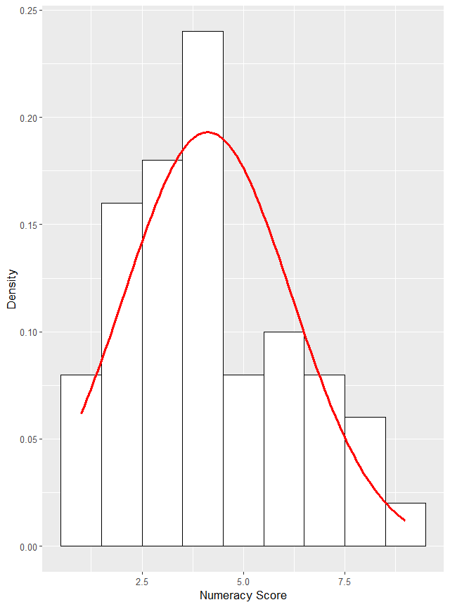
hist.numeracy.duncetown <-
    ggplot(dunceData, aes(numeracy)) +
    theme(legend.position = "none") +
    geom_histogram(aes(y = ..density..), fill = "white", colour = "black", binwidth = 1) +
    labs(x = "Numeracy Score", y = "Density") +
    stat_function(fun=dnorm, args=list(mean = mean(dunceData$numeracy, na.rm = TRUE), sd = sd(dunceData$numeracy, na.rm = TRUE)), colour = "red", linewidth = 1)
hist.numeracy.duncetown
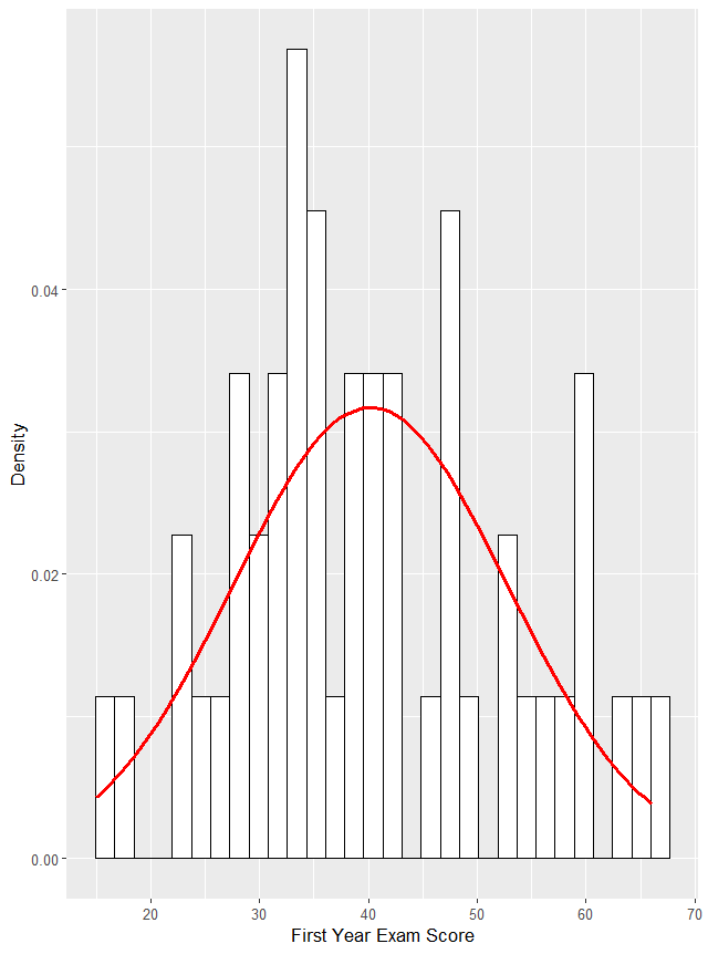
hist.exam.duncetown <-
    ggplot(dunceData, aes(exam)) +
    theme(legend.position = "none") +
    geom_histogram(aes(y = ..density..), fill = "white", colour = "black") +
    labs(x = "First Year Exam Score", y = "Density") +
    stat_function(fun=dnorm, args=list(mean = mean(dunceData$exam, na.rm = TRUE), sd = sd(dunceData$exam, na.rm = TRUE)), colour = "red", linewidth = 1)
hist.exam.duncetown
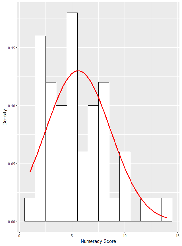
hist.numeracy.sussex <-
    ggplot(sussexData, aes(numeracy)) +
    theme(legend.position = "none") +
    geom_histogram(aes(y = ..density..), fill = "white", colour = "black", binwidth = 1) +
    labs(x = "Numeracy Score", y = "Density") +
    stat_function(fun=dnorm, args=list(mean = mean(sussexData $numeracy, na.rm = TRUE), sd = sd(sussexData$numeracy, na.rm = TRUE)), colour = "red", linewidth = 1)
hist.numeracy.sussex
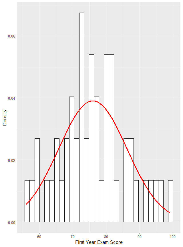
hist.exam.sussex <-
    ggplot(sussexData, aes(exam)) +
    theme(legend.position = "none") +
    geom_histogram(aes(y = ..density..), fill = "white", colour = "black") +
    labs(x = "First Year Exam Score", y = "Density") +
    stat_function(fun=dnorm, args=list(mean = mean(sussexData$exam, na.rm = TRUE), sd = sd(sussexData$exam, na.rm = TRUE)), colour = "red", linewidth = 1)
hist.exam.sussex
5.6. Testing whether a distribution is normal P217
5.6.1. Doing the Shapiro-Wilk test in R
N.B.: Not simply believe the test results, you should also plot the data (in histograms or qqplots) to see if it is normal
- Shapiro-Wilk test
- 把我们的数据与一个 normally distributed dataset 进行比较(这个 dataset 的 mean 和 sd 与我们数据的相同)
- 若结果 p<0.05, sign., 则我们的数据 non-normal
- 若结果 p>0.05, ns., 则我们的数据 normal
shapito.test()输出的W就是stat.desc()输出的normtest.Wp-value就是stat.desc()输出的normtest.p
#Shapiro-Wilks test for exam and numeracy for whole sample
shapiro.test(rexam$exam)
shapiro.test(rexam$numeracy)
#结果显示,exam和numeracy的shapiro-wilk test结果的p-value都显著< 0.05,说明这两个数据集都不是正态分布的,这也反映了exam 数据有两个modes,numeracy数据是positive skewed的事实

#但是,我们要是按组别来分别对不同uni的数据进行shapiro-wilk test,结果可能就与一饼巴的不同了
#Shapiro-Wilks test for exam and numeracy split by university
by(rexam$exam, rexam$uni, shapiro.test)
#可以看到这时两个uni的exam的test结果都> 0.05 说明数据分布都是normal的;这一点在组间比较中很重要

by(rexam$numeracy, rexam$uni, shapiro.test)
#而两个uni的numeracy数据却non-normal

#qqplots for the two variables
qqPlot(rexam$exam)
ggsave(file = paste(imageDirectory,"05 exam QQ.png",sep="/"))
qqPlot(rexam$numeracy)
ggsave(file = paste(imageDirectory,"05 numeracy QQ.png",sep="/"))
#从这两个qqplot我们能看到总体数据的exam和numeracy的数据分布是non-normal的,因为这些数据点没有与线重合

qqPlot(dunceData$exam)
qqPlot(sussexData$exam)
#而我们单看某个uni的exam数据,就比较normal了,所以要检查数据是否normal,要结合图与test result 一起看
5.6.2. Reporting the Shapiro-Wilk test
shapiro.test(rexam$exam)
#可以这样报告test结果:The percentage on the R exam, W = 0.96, P = .005, was significantly non-normal
Here2day